Appendix B — Part II Data Appendix: Harmonized Survey Data
This appendix documents the data underlying Part II’s quantitative analysis: the primary survey sources, the methodological decisions made while harmonizing them into a single analytic series, the resulting codebook, an external validation exercise, extended per-figure notes, and the steps required to reproduce the pipeline. It is self-contained so that it can travel with Part II if that chapter is developed into a standalone article (see sec-intro-notes’s index).
B.1 Data Sources
The quantitative analyses in Part II rely on the following primary data sources:
PNAD — Pesquisa Nacional por Amostra de Domicílios (Annual, 1992–2011). Collected by IBGE, this is a household survey providing annual microdata on income, education, and labor market outcomes. The rural North was excluded in 2004–2015 (Decision D03) for comparability with the PNAD of 1992–2003, which did not sample it; PNAD Contínua retains the rural North throughout, so the harmonized series carries a small coverage step in 2016 (about +0.4 pp on the national 18–24 access rate) alongside the instrument step (see the D03 addendum of 2026-09-19 in the decisions log).
PNAD Contínua — PNADC (2012–2025). The redesigned continuous household survey that replaced PNAD Anual. Uses a more complex sample design (rotating panels, stratified PSU sampling) requiring exact complex survey estimation via survey::svydesign().
Censos Demográficos (1960, 1970, 1980, 1991, 2000, 2010). Decennial censuses accessed via the censobr R package (v0.5.0), which provides harmonized Arrow parquet files. Microdata are cached locally after first download.
Salário mínimo — IPEADATA. Monthly minimum wage series used to deflate income brackets in historical censuses.
B.2 Methodological Decisions
Methodological decisions made during data harmonization are recorded in a numbered decision log maintained at docs/harmonization_decisions.md. The table below provides a summary of the most consequential decisions.
| Decision | Description |
|---|---|
| D01 | Deflate all monetary values to January 2024 prices using the IPCA (via deflateBR), applied at each survey’s reference date |
| D02 | Exclude observations with zero per capita household income (renda_dom_pcta == 0) |
| D03 | Exclude rural North (UFs 11–16) from PNAD Anual 2004–2015 for comparability with pre-2004 PNAD, which did not sample it; PNADC retains the rural North (coverage step of about +0.4 pp in 2016; addendum 2026-09-19) |
| D11 | Exclude 2020–2021 from the harmonized series (COVID-19 data methodology) |
| D19 | Tertiary enrollment indicator (ens_sup_a) = currently enrolled (not ever attended) |
| D20 | Treat the PNAD 1992–1999 non-declared-income sentinel code (V4722 == 999999999999) as missing at import, so that non-declared income is excluded alongside zero income (as D02 already stated) rather than silently ranked at the top of the income distribution |
| D21 | Retain the survey-specific unit of income aggregation across the splice — family in PNAD Anual, household in PNADC — rather than rebuilding the series on a single unit; sensitivity reported below |
| D22 | Course codes of PNAD Anual by dictionary regime (1992–99 / 2001–06 / 2007+): in 2001–2006 code 9 of V0603 is pré-vestibular and 10 is graduate study — the 1990s coding applied to those years had counted entrance-exam preparation as tertiary entry (corrected 2026-09-15; see sec-validation) |
| D21-B | Historical census education proxy: 1960 uses V213 (combined proxy); 1970 uses V038 (graduates only — not correctable; documented as limitation) |
| D27 | Decile assignment for variables with ≤ 9 distinct values: CDF-lower-bound method (decil = ceiling(cdf_lo × 10), clamped to [1, 10]). Applied to 1960 (8 midpoints). Full rationale in docs/audits/censo_historico_1960_1980.md. |
| D28 | Deciles, vintiles and quintiles in the harmonized PNAD/PNADC series (2026-09-19): each record is placed at the midpoint of its weight in the weighted income CDF within year × source, ties at income mass points (multiples of the minimum wage; 3.7% of the population at exactly 1 minimum wage per capita in 2025) broken by a fixed-seed draw, so that groups are balanced to within one record’s weight; replaces cut() on weighted quantile breaks, which left deciles up to 3.3 pp away from 10% of the population (1995). Fractional-rank concentration indices are unaffected |
B.3 Harmonized Analytic Datasets
The harmonization pipeline produces two analysis-ready parquet files, generated by R/01_pipeline/035_Splice_Microdados.R from intermediate PNAD Anual and PNAD Contínua (PNADC) extracts:
output/Microdados_Jovens_18_24_1992_2025.parquet(≈1.42 million rows) — the 18–24 age subset used for the main access-to-tertiary-education series.output/Microdados_Todas_Idades_1992_2025.parquet(≈12.0 million rows) — the full population with valid income, used for income-decile construction and robustness checks across age groups.
Universe and sample. Both files are restricted to individuals in households reporting strictly positive per-capita household income (Decision D02); PNADC is restricted to first-interview respondents only, to avoid the panel’s repeated-measurement structure inflating effective sample size. Excluding zero or non-declared income removes a modest share of the population, and the two categories are conceptually distinct: zero income is a declared value, whereas non-declared income (recorded in the 1992–1999 PNAD under a sentinel code; Decision D20) is unknown, so that assigning those individuals to any position in the income distribution would be an unfounded imputation. In 2001–2025 the combined exclusion ranges from 1.0 to 3.0 percent per year (peaking at 3.0 percent in 2011); in 1992–1999 it ranges from 4.9 to 6.5 percent per year, roughly half declared-zero and half non-declared income. Sensitivity to this exclusion is tested in R/02_validation/098_Sensitivity_Renda_Zero.R. The series covers 1992–1999, 2001–2009, 2011–2019, and 2022–2025: the years 2000 and 2010 are absent because no PNAD was fielded in census years, and 2020–2021 are excluded for documented data-quality reasons related to the pandemic-era PNADC redesign (Decision D11). The rural North (IBGE states 11–16) is excluded from PNAD Anual 2004–2015 for comparability with the PNADC’s initial geographic coverage (Decision D03), but is retained in PNADC, which raises PNADC access rates by approximately 0.4 percentage points relative to a fully matched geography.
Variables.
| Column | Type | Domain | Definition |
|---|---|---|---|
ano |
integer | 1992–2025 (with gaps) | Survey year |
idade |
integer | 0–130 (18–24 in the youth subset) | Age in years (PNAD V8005; PNADC V2009) |
peso |
double | >0 | Person-level sampling weight (PNAD V4729; PNADC V1028, first visit) |
renda_dom_pcta |
double | >0 | Nominal per-capita income of the respondent’s co-resident income unit, in the currency of the survey year (Cr$ 1992, CR$ 1993, R$ 1995+). The unit is the family in PNAD Anual (V4722/V4724) and the household in PNADC (VD5008); the two coincide exactly except where two or more families share a dwelling (Decision D21) |
renda_real |
double | >0 | renda_dom_pcta converted to R$ and deflated by the IPCA to January 2024 prices (Decision D01) |
ing_medio |
binary | 0/1 | Ever enrolled in secondary education. PNAD: current secondary/EJA-secondary/pré-vestibular enrollment, or prior course at or above colegial level, or years of schooling ≥ 9, or tertiary enrollment; PNADC: VD3004 ≥ 4 |
medio_completo |
binary | 0/1 | Completed secondary education. PNAD: years of schooling ≥ 11, or tertiary enrollment; PNADC: VD3004 ≥ 5 |
ens_sup |
binary | 0/1 | Ever enrolled in tertiary education — currently enrolled, graduated, or withdrawn; includes graduate study. This is the dissertation’s master access variable, validated against an external reference series to within ±0.3 percentage points nationally (sec-validation). It combines current-enrollment items with prior-enrollment items so that individuals who completed and exited tertiary education before the survey date are correctly counted as having accessed the system |
ens_sup_a |
binary | 0/1 | Currently enrolled in tertiary education (a subset of ens_sup) |
sup_completo |
binary | 0/1 | Completed tertiary education. PNAD: years of schooling ≥ 15 (standard proxy); PNADC: VD3004 = 7 |
decil |
integer | 1–10 | Income decile of renda_real, computed over the full population (not only youth), weighted, separately within each year × source (Decisions D08, D18, D28). D1 = poorest 10 percent |
vintil |
integer | 1–20 | As decil, in twenty groups |
fonte |
character | “PNAD Anual” / “PNAD Contínua” | Source survey. 2012–2015 exist in both sources (an intentional overlap retained to validate the splice); any analysis spanning these years must filter to a single source to avoid double-counting |
Logical hierarchy. By construction, and verified at build time: ens_sup_a ⊆ ens_sup ⊆ ing_medio, and sup_completo ⊆ medio_completo ⊆ ing_medio.
Known limitations. Income deciles and vintiles are computed within year and within source; they are comparable as relative positions across years, not as fixed income bands. Years of schooling in 1992–1995 carry 21–22 percent missing values in the underlying PNAD item, which slightly understates medio_completo and sup_completo in that window (missing values are coded 0 unless ens_sup independently indicates otherwise). The ing_medio variable shows a residual 5-percentage-point gap between PNAD and PNADC in the overlap years, reflecting genuinely distinct measurement instruments (a course-based questionnaire in PNAD versus the derived VD3004 indicator in PNADC); all other variables splice with a gap of 1.1 percentage points or less. For cohorts educated under the pre-1971 schooling structure, segundo ciclo (colegial/científico/clássico) counts as secondary completion while primeiro ciclo (ginásio) does not.
B.4 Validation Against an External Reference Series
The harmonized ens_sup series was benchmarked against the independent tertiary-access series of Salata et al. (2025), which covers an overlapping period using a different processing pipeline (DataZoom/Stata). The comparison script (R/099_Compare_vs_Salata.R) computes, for every year and income decile common to both series, the difference between the harmonized estimate and the reference estimate; the full year-by-year and decile-by-decile output is preserved in 4-DA-Code/2026-06_Harmonizing-BR-Data/docs/audits/AUDIT_REPORT_vs_Salata.md, with the underlying figure and table at 6-images-tables/graphs/2026-06-09_099A_Compare_Salata_vs_Harm.png and ..._099B_Diff_Salata_vs_Harm.csv.
An initial round of this comparison surfaced a coding error in the tertiary-enrollment variable for the PNAD Anual years (1992–2015): the original construction captured only currently-enrolled students, omitting respondents who had already completed or withdrawn from tertiary education, with the gap concentrated in the top income decile and growing over time (reaching −12.5 percentage points at D10 before correction). This was corrected by incorporating the PNAD items for prior school attendance and highest level previously attended (V0606/V0607, renamed V6007 from 2007 onward) into the ens_sup construction, matching the definition used by Salata et al. and now used in the published dictionary above.
After this correction, and after the course-code correction described below (Decision D22), the harmonized series and the reference series agree closely across the full 1992–2025 window:
| Period | Source | National difference (harmonized − Salata) | Assessment |
|---|---|---|---|
| 1992–1999 | PNAD histórica | −0.08 to +0.09 pp | Aligned |
| 2001–2003 | PNAD Anual | −0.16 to −0.04 pp | Aligned |
| 2004–2006 | PNAD Anual | +0.16 to +0.24 pp | Aligned — rural North exclusion (D03) |
| 2007–2011 | PNAD Anual | +0.22 to +0.33 pp | Aligned — rural North exclusion (D03) |
| 2012–2015 | PNAD Anual | +0.09 to +0.19 pp | Aligned |
| 2016–2019 | PNADC | −0.01 to −0.08 pp | Aligned |
| 2022 | PNADC | −0.71 pp | Acceptable — rural North retained in PNADC |
Three aspects of the comparison are worth recording explicitly. First, an earlier state of this table carried an excess of 1.5 to 1.7 percentage points for 2001–2006, which was then attributed to the exclusion of the rural North from PNAD Anual (Decision D03). That attribution was wrong, and a code audit on 2026-09-15 found the actual cause: the PNAD dictionaries of 2001–2006 code “pré-vestibular” (university entrance preparation) under the same code number that the 1992–1999 dictionaries use for graduate study, and the harmonization applied the 1990s coding to both regimes, so that entrance-exam preparation students were counted as tertiary entrants for six years (Decision D22). The mean age of respondents under that code — 22 in 2001–2006 against 35 in 1992–1999 — made the misreading visible once looked for. Correcting the code lowered the national 18–24 access rate by 1.3 to 1.8 percentage points in those years (up to 4.8 points in the top decile in 2001), removed a spurious step between 2006 and 2007 in the top-decile series, and brought the residual difference against Salata et al. to the values in the table. The residual now behaves exactly as D03 predicts: essentially zero in 2001–2003, when no survey sampled the rural North, and about +0.2 points from 2004 onward, when the IBGE began sampling it and D03 excludes it from PNAD Anual — the same order of magnitude as 2007–2015. The two readings could not be told apart from the national series alone; what separated them was that a coverage effect cannot exist in years without coverage. Second, the benchmarking exercise itself surfaced a data error in an earlier version of the pipeline: the top decile (D10) for 1992–1999 initially sat 3 to 5 percentage points below the reference series, while D9 sat a comparable margin above it. Tracing that residual revealed that the historical PNAD records non-declared family income under a sentinel code (999999999999) which the import step was converting to a numeric value, silently ranking roughly 2.5 percent of individuals with unknown income at the top of each year’s income distribution (Decision D20). After excluding those cases — the treatment D02 had always specified for non-declared income, and the same adopted by Salata et al. — the 1992–1999 top-decile series agrees with the reference to within 1.3 percentage points (within 0.5 points in five of the seven years), and the D9 excess disappears. Third, no artificial break was detected at the PNAD/PNADC splice point (2012–2015), where the two sources independently track the reference series within 0.4 percentage points of each other.
Averaged across the 26 years common to both series, the harmonized series is within 0.25 percentage points of the reference at every decile on average (the largest single-year departures being +1.2 points at D10 in 2004–2005 and −1.1 to −1.3 points at D10 in 1992–1993), and within 0.35 percentage points nationally in every year except 2022 — a level of agreement adequate to support the descriptive and counterfactual analyses in Part II. The post-correction comparison is recorded in 4-DA-Code/2026-06_Harmonizing-BR-Data/docs/audits/2026-09-15_Revalidacao_vs_Salata_pos_prevestibular.md.
One further asymmetry deserves recording, because it concerns the ranking variable on which every decile and every concentration index in Part II depends. The IBGE distinguishes the household (all co-residents) from the family (the subset related by kinship), and a household may contain more than one family: a young adult who has partnered and had children while continuing to live with their parents constitutes a second family under the same roof. The annual PNAD supplies income aggregated at the family level (V4722, divided by family size V4724), whereas the PNADC’s derived variable VD5008 aggregates at the household level. Both exclude the same categories of resident — lodgers, domestic workers, and their relatives — so the two measures coincide exactly in single-family households and diverge only where families are co-resident, a configuration whose incidence falls from roughly 11 percent of the population in the late 1990s to 7 percent by 2015. The series retains each survey’s native unit rather than rebuilding both on a common one (Decision D21), and the cost of that choice is bounded by direct measurement: reconstructing the household-level measure from the raw microdata for seven years spanning the series (V4721 divided by the count of residents outside the excluded categories) shifts the Wagstaff index by between +0.0008 and +0.0063, always in the same direction and without temporal drift, against a series that falls from 0.77 in 1995 to 0.53 in 2015. Between 8 and 15 percent of 18-to-24-year-olds change decile under the alternative measure, but almost always by a single decile and in both directions, so the shift very largely cancels in aggregation (the rank correlation between the two measures never falls below 0.978, and no decile’s access rate moves by as much as one percentage point). The bias is thus a level effect an order of magnitude smaller than the confidence intervals drawn in the figures, and it leaves the trajectory — the quantity the chapter actually reads — unaffected. Replication code: 4-DA-Code/2026-06_Harmonizing-BR-Data/R/02_validation/101_Sensitivity_Renda_Familiar_vs_Domiciliar.R.
B.5 Reproduction Guide
The full pipeline is documented in 4-DA-Code/2026-06_Harmonizing-BR-Data/README.md (bilingual, with dependency list and execution order); this section summarizes the essentials. Scripts are run from the thesis repository root, not from a sub-project, so that relative paths to 5-data/ resolve correctly.
The core extract-transform-load sequence runs three scripts in R/01_pipeline/: one importing PNAD Anual 1992–1999 from raw SAS-format microdata, one importing PNAD Anual 2001–2015, and 035_Splice_Microdados.R, which combines both PNAD extracts with the cached PNADC 2012–2025 first-interview extract (built separately in the 2026-05_PNADcIBGE project) into the two final parquet files described in sec-codebook. Decennial census validation points (1991, 2000, 2010), used only as cross-checks and not as part of the analytic series, are built separately via the censobr package.
Raw and intermediate microdata are not stored in the Git repository: they are downloaded or cached on first run into 5-data/ (maintained outside version control in the parent MancanoSync/ directory) because of file size. A fresh checkout therefore requires re-running the download steps before the harmonization scripts; cached files are reused on subsequent runs. Robustness checks (sensitivity to the zero-income exclusion, the rural North filter, and others) live in R/02_validation/; the figures used in the dissertation are produced by the scripts in R/03_analysis_plots/.
B.6 Alternative Specification: Access vs. Active Enrollment
The active-enrollment specification, documented in sec-fignote-delta-matriculados-decil-governo, measures change in active tertiary enrollment (ens_sup_a) — whether an 18–24-year-old is currently enrolled at the time of the survey. This criterion undercounts cumulative engagement with the system: a student who already graduated, or who withdrew after enrolling, no longer counts as “currently enrolled” even though they did access tertiary education. Readers who consider active enrollment too narrow a criterion for assessing distributive change can instead consult the figure below, which reproduces the identical decile-by-government design using ens_sup — whether an 18–24-year-old has ever accessed tertiary education (currently enrolled, graduated, or withdrawn; sec-codebook, the dissertation’s master access variable).
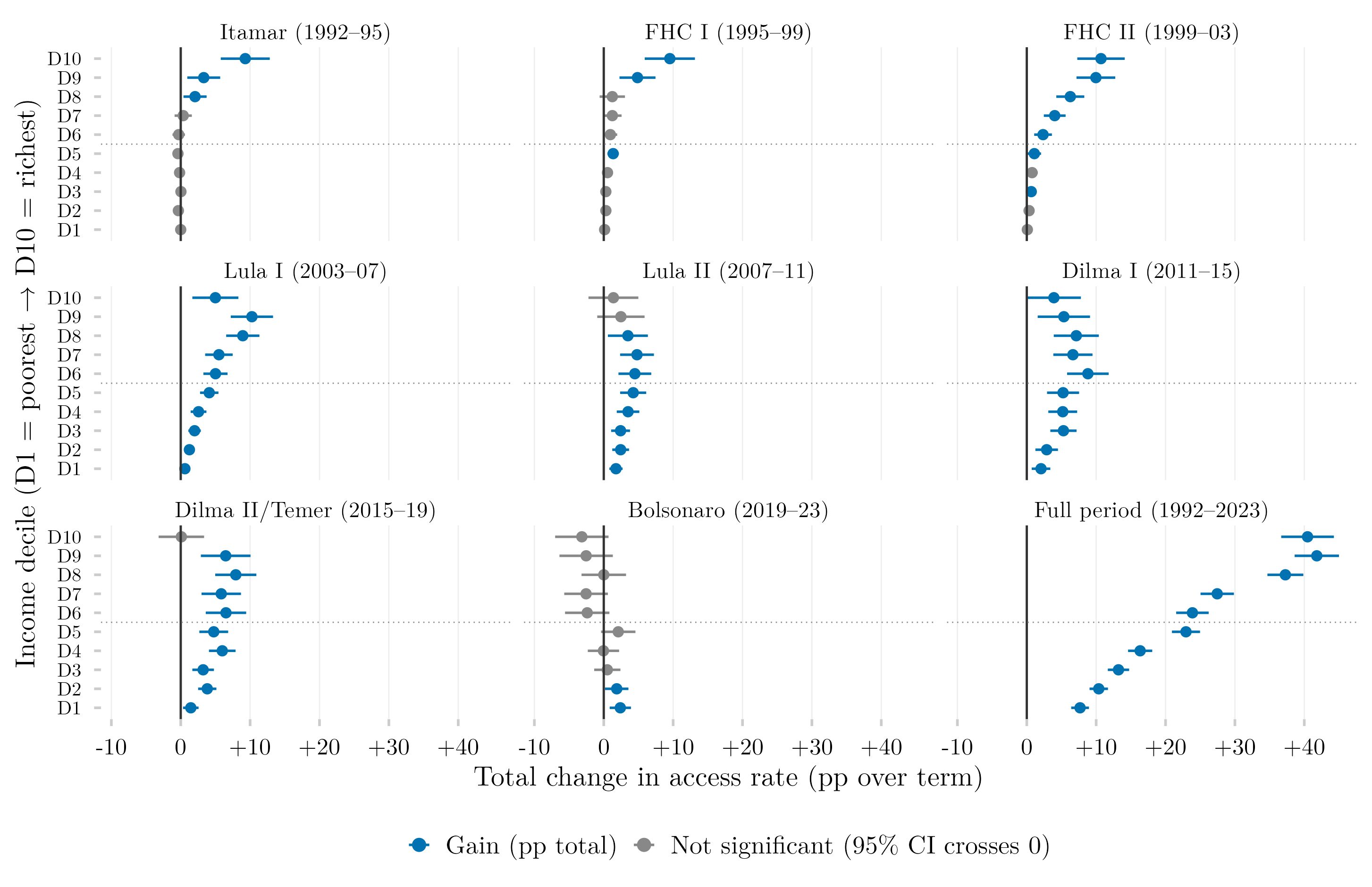
The access-based series tracks the same qualitative pattern as the active-enrollment series documented in sec-fignote-delta-matriculados-decil-governo — the same governments show gains or losses for the same deciles — but with larger absolute magnitudes throughout, since the access measure accumulates rather than resets: it does not lose cohorts who completed or withdrew. The full 1992–2023 period reaches +40.5 percentage points at D10 under the access criterion, against +29.1 under active enrollment. Replication code: 4-DA-Code/2026-06_Harmonizing-BR-Data/R/02_validation/042C_Tese_Dotplot_Acesso.R.
B.7 Replication of Senkevics et al. (2024)
Part II relies on Senkevics et al. (2024) for the claim that performance on the ENEM is itself strongly stratified by income and that the public and private sectors convert performance into enrollment in different ways. Because that study is the closest published counterpart to the dissertation’s own reading of the Brazilian case, its central figure was replicated on the same linked administrative data before being used as evidence. The replication follows the authors’ publicly released code (SAS, Stata and R) for every definitional choice — income midpoints, the cohort filter, the age window, the sector mapping and the first-enrollment rule — and departs from it only where the differential-privacy layer of the SEDAP+ platform makes the original operation impossible. The departures are catalogued in sec-replicacao-senkevics2024-design. The replicated figure is Figure fig-replicacao-senkevics2024-coortes, in which the 2012 cohort of the article appears in the lighter shade of each colour and the 2019 cohort, added by this dissertation, in the darker one.
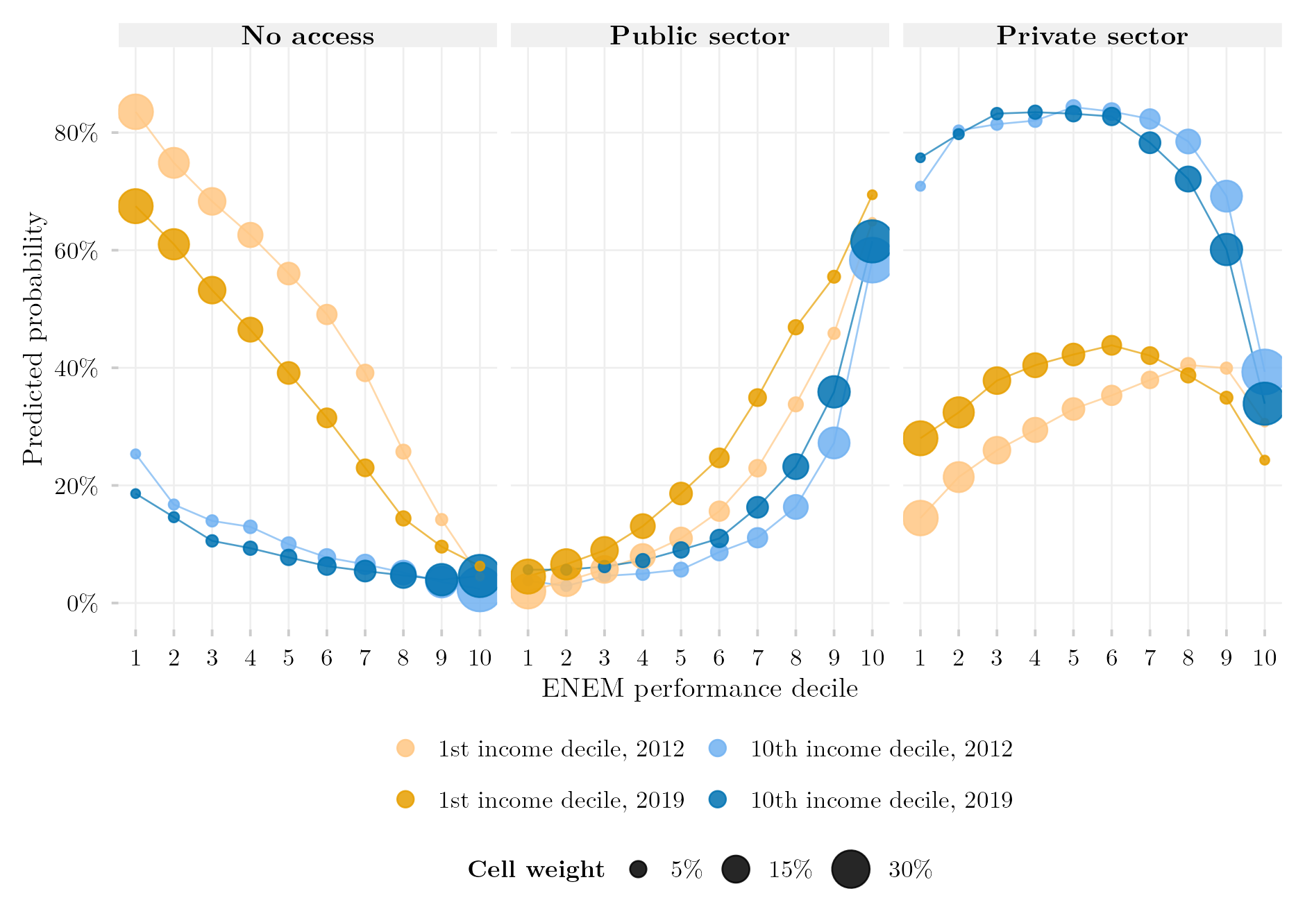
The 2012 cohort recovers the published marginals closely. Among entrants, 74.8% enrolled in the private sector and 25.2% in the public sector, against 75.8% and 24.2% in the article; 67.1% of the cohort entered some institution within five years, against 68.9%. The three patterns the authors read from the figure are all present in the lighter series: the probability of no access falls with performance for both income strata but from very different starting points; public-sector entry rises steeply with performance for both; and private-sector entry for the richest stratum forms a high, flat plateau across the middle of the performance distribution that the poorest stratum never approaches. The one visible divergence is in level rather than shape, and it is where the missing controls bite hardest: in the public-sector panel at the top performance decile, the replication places the poorest stratum above the richest (0.65 against 0.58), whereas the published figure, which conditions on sex, colour, age, school network, rurality, state and ENEM edition, places it below (roughly 0.40 against 0.57, read from the printed figure). Replication code: 4-DA-Code/2026-08_Replicacao_Senkevics2024/, scripts 010–040 for each cohort and 085 for the figure.
B.8 Extended Figure Notes
Since 2026-07-06, the in-chapter fignote under each figure is deliberately short (≤ ~5 printed lines; WRITING-STYLE.md §13.7): it states what the figure shows, the variable and cut, the confidence-interval method, and a link back here. This section is the second layer: one anchored subsection per figure, carrying the full methodological detail — harmonization decision codes, raw survey variable identifiers, source-splicing and estimation minutiae — that used to be repeated inside every fignote. Each entry cross-references sec-decisions, sec-codebook, or sec-validation for whatever is common to several figures, rather than restating it. Each entry closes with the address of the page in Open Data Analysis (sec-replication) that carries the code and pipeline reproducing the figure.
B.8.1 Tertiary Access by Income Decile, 1992–2025 (@fig-decil-acesso-serie-historica)
Each series shows the share of 18–24-year-olds who had ever enrolled in tertiary education (ens_sup, cumulative access; sec-decisions, Decision D19), by decile of per-capita household income and for the population as a whole. Deciles are computed within each survey year and source over the full population with strictly positive income, with ties at income mass points split by a fixed-seed draw so that each decile holds one tenth of the population (sec-decisions, Decisions D02, D08, D18, D28). The harmonized series uses PNAD Anual through 2015 and PNAD Contínua from 2016 onward, so that each year draws on a single source (sec-codebook); the rural North is absent from PNAD Anual 2004–2015 (Decision D03). Lines are interrupted in years without a survey: 1994 (no PNAD was fielded), 2000 and 2010 (census years, in which no PNAD was fielded) and 2020–2021 (excluded for pandemic-related data-quality reasons; Decision D11). Confidence intervals are 95% intervals: Wilson score intervals with the Kish effective sample size under a design effect of 2.0 for PNAD Anual (1992–2015), and design-based intervals from exact complex-survey estimation via survey::svydesign() (primary sampling units and strata) for PNAD Contínua (2016–2025). Diamonds mark independent validation points from the long-form samples of the 2000, 2010, and 2022 Demographic Censuses (via censobr; the 2022 sample via censobr::import_microdata22_controlado(), dev branch, commit dd48725); given the census sample sizes, their 95% confidence intervals span at most 0.6 percentage points for 2000 and 2010, and up to 0.7 percentage points for 2022 (widest at the top decile), in every case narrower than the diamond markers themselves, so they are not drawn. Validation points for the 1991 Census are also computed, but fall outside the plotted range (1992–2025) and do not appear in the figure; the 1991 census reports income in fourteen ordinal ranges, from which deciles are approximated, and the bracket boundaries leave no observations assigned to the third decile in that year (sec-decisions, Decisions D26, D27). Government labels indicate the president, abbreviated where the term block is narrow (D.II/Tem. = Dilma Rousseff’s second term joined to Michel Temer’s; Bolson. = Jair Bolsonaro; L. III = Lula’s third term). Reproduce: posts/decil-acesso-serie-historica/ (Open Data Analysis).
B.8.2 Relative Access Inequality, Wagstaff Index (@fig-wagstaff-intro)
Panel A. The Wagstaff concentration index (\(W\)) is a Gini-like scalar bounded for binary outcomes: \(W\) approaching zero indicates access has become de-commodified — independent of household income — while a high, positive \(W\) indicates access remains a commodity, allocated chiefly by ability to pay. \(W\) is computed via weighted survey GLM regression, a convenient parameterization of the concentration curve, under a uniform Kish design-effect approximation (\(\text{DEFF} = 2.0\)) across both PNAD Anual and PNAD Contínua to preserve longitudinal comparability across the instrument transition, whereas decile-specific access rates draw on exact complex-survey estimation in PNAD Contínua (sec-codebook for the source splice). Grey bands are 95% confidence intervals. Solid lines/circles denote ever accessed tertiary education (ens_sup); dashed lines/triangles denote currently enrolled (ens_sup_a; sec-decisions, Decision D19 for both). The labels along the top mark each presidential administration’s term, with a thin underline spanning its exact period — the reference implementation for the government-term band used across the dissertation’s time-series figures (WRITING-STYLE.md §13.8).
Panel B. The Gini index of household per-capita income, drawn from the same official IBGE series used throughout the dissertation’s income-inequality figures (238_Serie_Desigualdade_Oficial.R), validated against IBGE’s own published figures (mean deviation −0.0001). The vertical line marks the 2015/2016 PNAD Anual/PNAD Contínua splice; open circles mark the retroweighted, telephone-collected 2020–2021 PNAD Contínua, plotted but not asserted comparable to the rest of the series. Reproduce: posts/wagstaff-acesso-matricula/ (Open Data Analysis).
B.8.3 Decomposition of Tertiary Access Inequality into Eligibility and Transition (@fig-wagstaff-decomposicao-funil)
Estimator and population. All series use the same estimator as Figure fig-wagstaff-intro: the concentration index \(C = 2\,\mathrm{cov}(y, r)/\mu\) estimated by weighted survey GLM regression on fractional income ranks, under a uniform Kish design-effect approximation (\(\text{DEFF} = 2.0\)) across PNAD Anual and PNAD Contínua, with each year drawn from a single source (PNAD Anual through 2015, PNAD Contínua from 2016; sec-codebook). The population is 18–24-year-olds in households with strictly positive per-capita income (sec-decisions, Decision D02); the rural North is absent from PNAD Anual 2004–2015 (Decision D03) and 2020–2021 are excluded (Decision D11). The outcomes are completed upper secondary (medio_completo; Decision D19: eleven or more years of schooling or any tertiary enrollment in PNAD Anual, VD3004 \(\geq\) 5 in PNAD Contínua) and ever entered tertiary (ens_sup; Decision D19), the latter being the same quantity as the 18–24 ever-accessed line of Figure fig-wagstaff-intro, recomputed by the same code on the same data.
The identity. For a binary outcome \(y\) ranked by \(r\), \(\mathrm{cov}(y, r) = \mu_y\,(E[r \mid y = 1] - \tfrac{1}{2})\), so that \(C_y = 2\,E[r \mid y = 1] - 1\): the concentration index is twice the mean income rank of those who have the outcome, minus one. Because ens_sup is nested within medio_completo by construction (the hierarchy ens_sup_a \(\subseteq\) ens_sup \(\subseteq\) medio_completo is enforced by the harmonization script; Decision D19), the mean rank rises in steps along the funnel and the sum telescopes: \[C_{\text{sup}} \;=\; \underbrace{2\,\big(E[r \mid \text{EM}] - \tfrac{1}{2}\big)}_{C_{\text{EM}}} \;+\; \underbrace{2\,\big(E[r \mid \text{sup}] - E[r \mid \text{EM}]\big)}_{T} ,\] where \(r\) is the fractional rank in the full 18–24 cohort, kept for completers rather than recomputed within them. The first term is the ordinary concentration index of upper secondary completion (the eligibility component); the second, \(T = 2\,\mathrm{cov}(t, r \mid e = 1)/\mu_{t \mid e}\), is the concentration of tertiary entry among completers measured on the full-cohort ranks (the transition component). The identity holds exactly and is verified numerically in the figure script (maximum absolute error \(1.6 \times 10^{-14}\) across years, with the two mean-rank readings verified to the same precision). The Wagstaff normalization is applied by dividing both components by the same \(1 - \mu_{\text{sup}}\) as the total, so that the plotted series still sum to \(W_{\text{sup}}\) and the share of each component, \(C_{\text{EM}}/C_{\text{sup}}\), is the same in \(C\) and in \(W\). The transition term is estimated by the same convenient regression as the other indices, run on completers only, with the rank variable held at its full-cohort values and the dependent variable scaled by the weighted variance of that rank within completers rather than by the variance of a uniform rank; this is what makes the coefficient equal to \(T\) rather than to a re-ranked index.
Two properties of the decomposition. First, it is a sequential attribution in the order of the funnel: the eligibility component is what the tertiary index would be if the transition among completers were income-neutral (\(E[r \mid \text{sup}] = E[r \mid \text{EM}]\) implies \(T = 0\) and \(C_{\text{sup}} = C_{\text{EM}}\)), and the transition component is what the second step adds. Reversing the order, by asking first what the index would be if eligibility were income-neutral, would give a different split; the order used here follows the actual sequence of the two transitions. Second, the transition component is a contribution rather than a bounded index. Its ceiling depends on the dispersion of completers along the full-cohort income distribution, which is small when completers are concentrated at the top (in 1992 they sat on average at the 74th percentile) and approaches the dispersion of a uniform rank as completion becomes general (in 2025 completers are 73.6% of the cohort). It can therefore be small even when the income gradient of entry among completers is steep, and it should not be compared with a standard concentration index computed on re-ranked completers.
Reading. In \(W\) units, the eligibility component falls from 0.50 in 1992 to 0.15 in 2025 and the transition component rises from 0.22 to about 0.37 in 2004–2006, falls to 0.29 in 2014 and settles around 0.32 thereafter; the two cross in 2004. The eligibility share of the tertiary index is 70% in 1992, 50% in 2004, 45% in 2009 and 31% in 2025. In percentile terms, completers moved from the 74th to the 55th percentile of the cohort and entrants from the 84th to the 66th, so that the eligibility distance shrank from 24 to 5 percentile points while the transition distance was 10 points in 1992, 16 in 2004 and 11 in 2025. The two readings differ in the recent level of the transition component because the Wagstaff normalization inflates both components as \(\mu_{\text{sup}}\) grows; in unnormalized \(C\) the transition term is 0.20 in 1992 and 0.22 in 2025. The 1992–1995 readings quoted here are subject to the V4703 coverage caveat below and should not be read substantively.
The conditional series with recomputed ranks. An earlier version of the chapter presented in its body the standard conditional concentration index: the sample restricted to upper secondary completers, the fractional income ranks recomputed within that subpopulation, and \(W\) of ever entering tertiary estimated on that basis. That series is retained here as Figure fig-wagstaff-transicao-condicional because it answers a question of its own, namely how concentrated entry is among the eligible when the eligible are treated as the whole population, which is the question closest to the second hypothesis of Salata et al. (2025). It is not, however, a component of the tertiary index, and its distance to the full-cohort tertiary series should not be read as the part of access inequality attributable to eligibility: the two indices are computed on different populations, with different ranking variables and different normalizing denominators (\(1 - \mu_{\text{sup}}\) against \(1 - \mu_{t \mid e}\), 0.94 against 0.65 in 1992), so that no identity links their difference to anything, and the apparent share of eligibility would have been 38% in \(W\) and 57% in \(C\) for the same year. The re-ranking is what breaks the additivity. Rewriting each covariance as a slope times the variance of its ranking variable, the re-ranked index uses the variance of a uniform rank (\(1/12\)) while \(T\) uses the variance of the full-cohort rank among completers, which is far smaller when completers are concentrated at the top; the two therefore diverge most when eligibility is most unequal (0.29 against 0.20 in 1992) and converge as completion becomes general (0.23 against 0.22 in 2025).
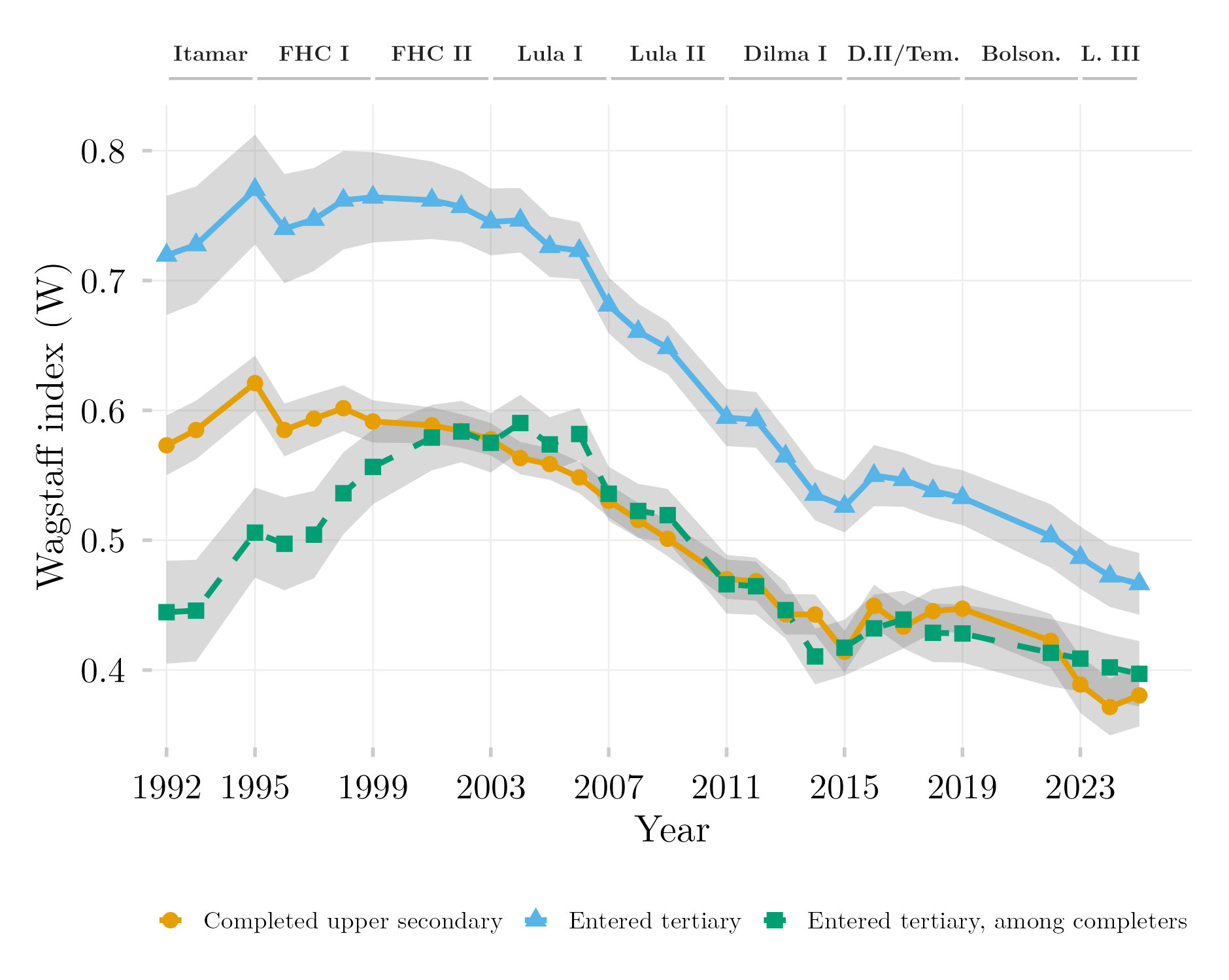
Conditioning on completion is conditioning on an outcome that itself depends on income, and the pool of completers grows from 17.6% of the cohort in 1992 to 73.6% in 2025, so the re-ranked series mixes changes in the transition with changes in who is eligible: it is descriptive and does not identify the effect of any policy. Its chronology matches that of the transition component in the main figure in its principal phases (rise, fall from 2007 to 2014, stability since 2015), with the difference that its rise flattens earlier: both series plateau over 2001–2006, the re-ranked index peaking in 2004 and the transition component in 2006. A second exact decomposition, linear in the outcome for a fixed ranking, splits the index of upper secondary completion into a term for those who went on to tertiary and a term for those who did not, weighted by their shares among completers (\(C_{\text{EM}} = (\mu_{\text{sup}}/\mu_{\text{EM}})\,C_{\text{sup}} + (\mu_{\text{EM only}}/\mu_{\text{EM}})\,C_{\text{EM only}}\), verified to \(4 \times 10^{-14}\)). The tertiary term accounted for half of the completion index in 1992 and for more than all of it from 2018 onward, since the concentration index of completing upper secondary without entering tertiary fell from 0.36 in 1992 to 0.04 in 2014, crossed zero in 2017–2018 and reached $-$0.06 in 2025, so that the completion index now carries little content beyond the tertiary index it contains. The diagnostic that establishes this, with the same series for ages 25–64 (not plotted; the adult conditional series is nearly flat, as expected of a stock that changes only by cohort replacement), is 4-DA-Code/2026-06_Harmonizing-BR-Data/R/02_validation/097F_Diag_Wagstaff_Transicao_Decomposicao.R; the figure script for the re-ranked series (097G_Tese_Wagstaff_Transicao_Condicional.R) reads its cached results.
Measurement caveats. In 1992–1995 the years-of-schooling variable behind medio_completo in PNAD Anual (V4703) is missing for roughly 21–22% of respondents and is coded as not completed unless ens_sup is one, which biases the pool of completers toward tertiary entrants in those years and affects both the eligibility component and the transition component; the first four years should not be read substantively. The 2015/2016 instrument splice is visible as a step in the full-cohort tertiary series and in both components, so the level shift around 2016 is at least partly an artefact of measurement. Government labels follow the conventions of sec-fignote-decil-acesso-serie-historica. Replication code for the two main figures: 4-DA-Code/2026-06_Harmonizing-BR-Data/R/02_validation/097H_Tese_Wagstaff_Decomposicao_Funil.R, which recomputes all terms from the harmonized microdata and stops if the identity fails to close. Reproduce the re-ranked series: posts/wagstaff-transicao-condicional/ (Open Data Analysis).
B.8.4 Change in Enrollment by Decile and Presidential Term (@fig-delta-matriculados-decil-governo)
Each point shows the total percentage-point change in the share of 18–24-year-olds actively enrolled in tertiary education (ens_sup_a), from the first year of each presidential term to the first year of the next; horizontal lines are 95% confidence intervals. Color encodes significance rather than sign: a point is grey wherever its interval contains zero, so that a change of half a percentage point indistinguishable from none does not carry the same visual weight as one of fifteen, and blue and orange are reserved for gains and losses whose intervals lie entirely on one side of zero. The interval is that of the difference itself, with its standard error taken as the root of the sum of the two years’ squared standard errors, which treats the two surveys as independent; the test is therefore conservative twice over, since it also inherits the design-effect penalty on PNAD Anual and ignores the correlation between waves of the PNAD Contínua panel. Confidence intervals for the underlying rates are computed via Kish design-effect approximation (PNAD Anual) and exact complex-survey estimation via survey::svydesign() (PNAD Contínua). Because each point is a difference rather than a level, the two source surveys are spliced by presidential term rather than by year: every term panel draws on a single survey at both of its endpoints, PNAD Anual through 2015 and PNAD Contínua from 2015 onward, so that no difference shown here straddles the change of instrument and silently adds the discontinuity between the two questionnaires — and between the family and household bases of the per-capita income variable (sec-decisions, Decision D21) — to the change it reports. The years 2012–2015 are carried by both surveys, which is what makes this possible; 2015 accordingly enters as PNAD Anual at the close of the Dilma I panel and as PNAD Contínua at the opening of the next, so the level at which one panel ends is not the level at which the following one begins. The full-period panel in the bottom-right corner is the single comparison no one survey spans, and is the only one that remains cross-survey. Panels are ordered chronologically left to right, top to bottom. Active enrollment is a conservative criterion that excludes cohorts who already graduated or withdrew; readers who consider this criterion too narrow can consult the alternative specification using ever-accessed status in sec-access-alt. Reproduce: posts/delta-matriculados-decil-governo/ (Open Data Analysis).
B.8.5 Median Household Income per Capita (@fig-renda-mediana-domiciliar-pc)
The series plots the weighted median of real per-capita household income, in January 2024 reais deflated by the IPCA (sec-decisions, Decision D01), for the population as a whole. The median is reported rather than the mean because the argument of this chapter concerns the income available to the household at the middle of the distribution, which the mean overstates: over the period covered here the mean runs between 1.5 and 1.7 times the median, and its movement is sensitive to the top decile in a way the barrier argument does not require.
Construction, and why it departs from the main harmonized panel. This figure does not read the analytic parquet that supplies the decile and concentration figures. It is built by a dedicated extraction from the raw microdata, for two reasons that matter for a level series and not for a distributional one. First, the unit of income is the household throughout: for PNAD Anual (1992–2015) the numerator is V4721, the IBGE household income aggregate, which by construction excludes the income of lodgers, domestic workers and their relatives, and the denominator is the count of residents outside those same three conditions (V0401 not in 6, 7, 8); from 2016 the PNAD Contínua supplies VD5008, which is already per-capita household income on the same convention. The main panel instead carries family income per capita until 2015 and household income from 2016 (Decision D21), an asymmetry adopted there because its effect on the Wagstaff index is between 0.0008 and 0.0063, an order of magnitude below the confidence bands; on a median the same asymmetry is worth several percentage points, because the family is a smaller and more homogeneous unit and the substitution moves precisely the middle of the distribution. Second, the universe is the official one, retaining households that report no income, as the IBGE convention does and as sec-validation already adopts for the Gini and Palma series; excluding them, as Decision D02 does for the decile analysis, raises the median by 4.9% in 2003, 2.4% in 2009 and 1.4% in 2014, since the excluded households sit below the middle. Neither departure affects any other figure in this thesis: D21 and D02 remain in force wherever the quantity of interest is relative position rather than level, and the two universes are kept apart deliberately, each fitted to what it measures.
Years without a comparable observation. The line is interrupted in 1994, 2000 and 2010, when no PNAD was fielded. The hollow markers for 2020 and 2021 are drawn from the fifth visit of the PNAD Contínua, the only annual file available for those years, collected substantially by telephone; the mode is known to under-enumerate income and to under-represent poorer and rural households without a telephone line, and the two points should be read as indicative rather than comparable to the rest of the series (sec-decisions, Decision D11).
The change of survey in 2015–2016. The solid vertical rule marks the point at which the series passes from PNAD Anual to PNAD Contínua. The step is not rescaled away. Its size was measured on the four years both surveys cover: with the unit of income made homogeneous on both sides, the PNAD Contínua median runs 5.0%, 4.1% and 3.7% below the PNAD Anual median in 2012, 2013 and 2014 and 0.8% above it in 2015, an average of −2.6%. Readers comparing levels across the rule should carry that figure in mind. A defensible alternative would be to rescale the older series by a splice factor estimated on the overlap, as Souza & Hecksher (2026) do; the choice here is to leave the series as a direct reading of each survey, consistent with every other series in this thesis, and to state the discontinuity rather than absorb it.
Provenance and acknowledgement. The household construction described above follows the procedure documented in the replication package that Pedro H. G. Ferreira de Souza and Marcos Hecksher released with Souza & Hecksher (2026), which Souza made available to me, to which I’m very grateful; the package supplies the harmonization routines for both surveys, the deflation convention, and intermediate results at annual frequency. The reading of the raw PNAD files, including the household identification key, reuses the machinery written for the sensitivity exercise reported in sec-decisions, Decision D21. Replication code: 4-DA-Code/2026-06_Harmonizing-BR-Data/R/02_validation/242_Tese_Renda_Mediana_Domiciliar.R, which caches the extracted series and, when the replication package is present, prints the year-by-year comparison against it. Reproduce: posts/renda-mediana-domiciliar-pc/ (Open Data Analysis).
B.8.6 Mean Household Income by Percentile (@fig-renda-media-centil)
Each line shows the weighted mean real per-capita household income (deflated to January 2024 prices via the IPCA from each survey’s reference month; sec-decisions, Decision D01) within each income percentile group, for six years chosen at five-year intervals from a continuous annual series (2002, 2007, 2012, 2017, 2022, 2025). Percentiles rank all individuals by income using sampling weights: each individual is assigned the centile given by the ceiling of the weighted cumulative population share multiplied by 100. Centiles 1 and 100 are excluded because of sampling instability at the extremes. For 2012, a year the harmonized series carries in both source surveys, only the PNAD Anual sample is used (sec-codebook). The y-axis is truncated at R$8,000; only the top one or two centiles of each year exceed this limit, falling substantially above it.
Same base as the median series. Since 2026-09-16 this figure no longer reads the analytic parquet. It is built on the same extraction as Figure fig-renda-mediana-domiciliar-pc (sec-fignote-renda-mediana-domiciliar-pc): household income per capita throughout, from the raw PNAD files for 2002, 2007 and 2012 (V4721 over the residents outside the lodger, domestic-worker and relative-of-domestic-worker conditions, read by R/utils/renda_domiciliar_pnad.R) and from VD5008 in the consolidated PNAD Contínua for 2017, 2022 and 2025, retaining households that report no income. The earlier version inherited from the parquet the family unit until 2015 (Decision D21) and the exclusion of zero-income households (Decision D02); measured against the present base, the family unit alone was worth about −2.3% in the middle of the distribution in the PNAD years, and the exclusion of zeros −10% to −13% at the 5th centile and almost nothing above the 30th, so the two conventions moved the two sides of the 2015–2016 survey change by different amounts — an asymmetry that does not matter for a figure of relative position but does for one of levels in reais. The script carries a lock that compares the median of its own base with the cached series of Figure fig-renda-mediana-domiciliar-pc year by year and stops if they diverge by more than 0.5%; they agree to within rounding in all six years, so the median of that figure is the 50th centile of this one. Setting MANTER_ZEROS <- FALSE reproduces the Decision D02 universe if ever needed.
Minimum-wage markers. Open circles mark the percentile whose mean income is closest to one (1 MW), one-and-a-half (1.5 MW) and three (3 MW) times the national minimum wage in force in the survey’s reference month — September for PNAD Anual, mid-June for PNAD Contínua — deflated from that same date, so that the marker and the incomes it is placed against share one price basis. The reference month matters before 2009, when the minimum wage was still readjusted in April: the wage of January 2002 (R$180) and January 2007 (R$350) was not the one in force when the survey was fielded. Nominal values used (IPEADATA series MTE12_SALMIN12): 2002 R$200; 2007 R$380; 2012 R$622; 2017 R$937; 2022 R$1,212; 2025 R$1,518 — or, at January 2024 prices, R$716, R$961, R$1,205, R$1,316, R$1,285 and R$1,415. The 1 MW marker sits at centiles 57, 60, 57, 61, 58 and 53 across the six years; the 1.5 MW marker at centiles 72, 76, 75, 78, 75 and 73; the 3 MW marker at 88, 91, 92, 92, 92 and 90. Read against each year’s own minimum wage, the position of each multiple in the distribution is therefore stable over the period, with a modest fall in the last year: what expanded was the real value of the wage itself (+97.7% between 2002 and 2025), not the fraction of the population above it. Reproduce: posts/renda-media-centil/ (Open Data Analysis).
B.8.7 Higher-Education Tuition vs. Consumer Prices and the Minimum Wage (@fig-ipca-mensalidade-curso-superior)
Both series track the higher-education tuition subitem of the IPCA, Brazil’s headline consumer price index, spliced from the four vintages of the subitem-level SIDRA series (tables 655, 2938, 1419, and 7060; the subitem is named Curso terceiro grau in 1999–2006 and Ensino superior thereafter) and expressed as a cumulative index with August 1999 = 100, the first month of the continuous post-stabilization series. The blue series deflates cumulative tuition readjustments by the headline IPCA (table 1737): values above 100 indicate that tuition rose faster than overall consumer prices after August 1999. The orange series divides the same tuition index by the nominal minimum wage (IPEADATA series MTE12_SALMIN12), measuring how the cost of the same tuition bill evolved relative to the wage floor — the more policy-relevant measure of affordability at the bottom of the income distribution. The step-like pattern reflects readjustments clustered at the start of each academic year (blue) and the annual minimum-wage adjustments (orange). The IPCA subitem is a price-change index computed over a fixed panel of institutions surveyed by the SNIPC in metropolitan areas, for households earning 1–40 minimum wages: it measures readjustment, not the price level or the average market ticket, and it does not capture compositional cheapening through the migration of enrollment toward distance learning and lower-priced institutions, so a falling market average ticket can coexist with this index rising. In real terms, tuition tracked or exceeded headline inflation until 2020 (peaking roughly 12% above the 1999 level) and fell below the 1999 benchmark only after the nominal tuition cuts of 2021 (annual readjustment of −1.0%); relative to the minimum wage, tuition fell by roughly 60%, with almost all of the decline concentrated in 2001–2012, the period of sustained real minimum-wage increases. Reproduce: posts/ipca-mensalidade-curso-superior/ (Open Data Analysis).
B.8.8 Seats Allocated by Targeted Access Policy (@fig-vagas-focalizadas)
Built by 4-DA-Code/2026-02_CENSUP_Public/047_Tese_Vagas_Focalizadas.R from a course-level aggregate of INEP’s Censo da Educação Superior: 2009–2023 are read from that aggregate unchanged, and 2024 is added from the public course file with the same recipe (sector from TP_CATEGORIA_ADMINISTRATIVA, 1–3 public; ProUni as the sum of full and partial scholarships; reserved seats from QT_MAT_RESERVA_VAGA). None of the PNAD/PNADC decisions catalogued in sec-decisions apply, since the unit is the institutional enrollment record rather than the household, and the series begins in 2009 because that is the first year of CENSUP microdata with enrollment-level flags for ProUni, FIES and reserved seats.
Sector attribution and its noise. ProUni and FIES are legally private-sector instruments and reserved seats a public-sector one, but the microdata records small counts against the wrong sector in most years: ProUni in public institutions (884 in 2009, 1,917 in 2011, single or double digits elsewhere), FIES in public institutions in every year from 2010 (peaking at 5,848 in 2017), and “cotista” enrollments in private institutions (2,149 to 12,043, peaking in 2013). These are treated as reporting error: ProUni and FIES are counted in the private network only and quota places in the public network only. The difference against the unrestricted totals is below 0.03 percentage points in every year, and the generating script prints the full noise table on each run.
What the stack counts. One could ask how much of the system carries no price, which would mean counting the whole free public network and keeping quota seats in a separate panel, since a reserved seat changes who occupies a free place rather than what it costs. This figure asks a narrower question — how much of the system is allocated by a need-based criterion — and for that question the three instruments belong in one stack: a reserved seat, a ProUni scholarship and a FIES contract are each assigned on public-school origin, family income, race or disability. Open-competition public seats, which are free but not targeted, are excluded. The two readings are not additive and should not be read against each other’s denominator.
What the series shows. The targeted share rises from 9.2% of enrollment in 2009 to 27.7% in 2016 and falls back to 12.1% in 2024; almost all of the bulge is FIES, which peaks at 1.34 million contracts in 2015 and ends at 155 thousand. The no-debt portion (quota seats plus ProUni) rises from 7.0% to 13.7% in 2019 and settles at 10.5%. Within it the composition inverts: ProUni falls from 616 thousand (2019) to 435 thousand (2024), while quota enrollment grows monotonically from 85 thousand to 642 thousand and has been the largest of the three instruments in absolute terms since 2021. The post-2019 decline in the shares is partly denominator growth — total enrollment rose from 8.6 to 10.2 million over 2019–2024 — and Panel B is provided so that the absolute movements can be read directly.
One limit specific to the quota series. QT_MAT_RESERVA_VAGA counts every student enrolled through any reservation programme the Census records — public-school, income, race, disability and “other” — including institutional programmes that predate Law 12,711/2012. The subtype fields (QT_MAT_RV_*) exist in the microdata but are not carried in the aggregate, so the figure cannot separate the federal quota law from earlier and state-level schemes.
Two limits on the shares. First, ProUni and FIES are treated as disjoint, but a student may hold a partial scholarship and finance the remainder, so the subsidized block is marginally overstated in the FIES peak years; the microdata do not permit separating the overlap. Second, every quantity is a share, so movements in the denominator matter: public enrollment was roughly flat near 2.05 million from 2019 onward while the total rose from 8.3 to 10.0 million, and the 2023 total alone jumped 5.6% over 2022, the largest single-year increase in the series. A substantial part of the post-2019 fall in every share is therefore denominator growth rather than contraction of the instruments, and should not be read as policy retreat alone. The 2020 dip in public enrollment (2,034,834 → 1,929,995 → 2,055,197) is a collection artifact of the pandemic year and is not a substantive inflection. Reproduce: posts/vagas-focalizadas/ (Open Data Analysis).
B.8.9 Enrollment by Sector, Access Route and Time of Day (@fig-matriculas-turno-via-acesso)
Built by 4-DA-Code/2026-08_SEDAP/050_Plot_Nicho_100pct_SEDAP.R from nicho_agregado_sedap_2010_2024.csv, which is extracted by 020_Extrair_Nicho_2020_2024.R from the student-level records of the Higher Education Census. Sector follows TP_CATEGORIA_ADMINISTRATIVA (1–3 public, 4–7 private). Access route is assigned by precedence within the private sector — ProUni first, then FIES among those without ProUni, then open admission — so the categories are disjoint by construction and a student holding a partial scholarship alongside a loan is counted once, as ProUni. Within the public sector the split is reserved seat versus open admission, where “reserved seat” means the reservation block of the record is filled at all, not merely that the public-school criterion is flagged; using the narrower flag would drop students admitted on income, race or disability criteria.
Why the source is SEDAP+ rather than the published microdata. SEDAP+ (Serviço de Acesso a Dados Protegidos) is INEP’s protected-access platform for educational microdata, launched in 2026 and reached at https://plataformasedap.inep.gov.br/; access is granted per research project, and the queries reported here were run under a project approved on 2026-04-29. INEP stopped publishing the student-level file of the Higher Education Census after 2019; from 2020 the public packages contain only the institution and course files, and the course file records shift and financial aid as separate marginals that cannot be crossed with one another. The series is therefore drawn from SEDAP+, INEP’s protected-access platform, for every year — including those where a public file exists — so that no year is measured on a different basis from another. A parallel extraction from the public files was used to validate the result and is retained in the generating code.
What the protected-access platform does to the numbers. SEDAP+ answers only aggregate queries and applies differential privacy, which in practice means it suppresses cells containing few individuals rather than adding appreciable noise: repeating the same query with the privacy parameter set to 1, 10 and 100 moved the total by 78 enrollments in ten million (0.0008%). Suppression, by contrast, is consequential when the grouping is fine — a five-column grouping lost 7 of 116 cells, about 113,000 enrollments — so the extraction groups at exactly the granularity the figure displays, at which no cell is suppressed. Against the published microdata for 2010–2019 the SEDAP+ totals run 0.6% to 1.1% low, a systematic and small gap; the ratios that carry the argument agree far more closely, with aid coverage in distance study at 5.2% against 5.3% and in-person at 24.1% against 24.0% for 2019. Two schema details are worth recording for anyone re-running the extraction: TP_CATEGORIA_ADMINISTRATIVA is stored as text in the early years and as an integer in the recent ones, and the aggregate reservation flag IN_RESERVA_VAGAS is entirely null from 2024, so the subtype fields must be used instead. The year 2009 is excluded because its time-of-day variable returns a single value.
One classification trap, recorded because the variable name invites it. IN_FINANCIAMENTO_ESTUDANTIL marks any student financing whatsoever, including institutional discounts and scholarships granted by the institution itself, which distance providers award on a large scale. Inferring ProUni as the residual of that flag minus FIES yields roughly 2.85 million scholarship holders for 2024, six times the size of the program. The nominal ProUni fields are the only reliable measure.
The color scheme carries an argument. With fifteen combinations, hue is assigned to sector crossed with access route and lightness to time of day, so that a color can be decoded positionally from the legend map rather than matched against a fifteen-item list. Distance learning departs from that rule deliberately: it receives a color family of its own rather than the darkest shade of its base hue, because it belongs analytically with the affordability channel rather than with the access routes. It lowers the income barrier in the way a subsidy does, through price, without being a policy — and displaying it as a shade of the route would have implied it was one more route.
Two cautions on reading the columns. First, the quantity is enrollment stock, not entrants, so a route’s share reflects the accumulated cohorts studying under it rather than the flow admitted in that year; the FIES collapse after 2015 therefore appears gradually as financed cohorts graduate or drop out, and its true inflection in admissions is sharper than the figure suggests. Second, quota enrollment before 2013 is small but nonzero, reflecting institutional reservation policies that predate the 2012 federal law (notably UERJ from 2003), so the series does not begin at zero and should not be read as though the law created reserved seats from nothing. Reproduce: posts/matriculas-turno-via-acesso/ (Open Data Analysis).
B.8.10 Secondary Education Completion by Income Decile (@fig-em-conclusao-decil)
Each series shows the share of 18–24-year-olds who completed secondary education (medio_completo), by decile of per-capita household income and for the population as a whole. Same recipe as Figure fig-decil-acesso-serie-historica: deciles computed within each survey year and source over the full population with strictly positive income, ties at mass points split by a fixed-seed draw (sec-decisions, Decisions D02, D08, D18, D28); the harmonized series uses PNAD Anual through 2015 and PNAD Contínua from 2016 onward (sec-codebook); lines are interrupted in years without a survey (1994; 2000, 2010 census years; 2020–2021, Decision D11). Confidence intervals: 95% Wilson score intervals with the Kish effective sample size (design effect 2.0) for PNAD Anual, and design-based intervals from exact complex-survey estimation for PNAD Contínua. Unlike Figure fig-decil-acesso-serie-historica, this figure has no independent census validation points: the census cross-check series maintained by this project (Censo_Pontos_Validacao_1991_2000_2010.parquet) was built only for the tertiary-access variable ens_sup and benchmarked against Salata et al. (2025) in sec-validation; building an equivalent census-based proxy for secondary completion (in the manner of the D21-B/D26/D27 decisions for the 1960–1991 censuses) was out of scope for this figure and is noted here as a limitation rather than silently omitted. Reproduce: posts/em-conclusao-decil/ (Open Data Analysis).
B.8.11 Income Inequality in Enrollment by Network Type, Wagstaff Index (@fig-wagstaff-rede-publica-privada-timeseries)
The Wagstaff index (W = CI / (1 − μ)) normalizes the Kakwani Concentration Index by prevalence (μ) — comparable across series with very different access rates (the public network has much lower prevalence than the private network among the 18–24 population: μ rises from 2.7% to 7.1% of that population over 2001–2025, more than doubling). Shaded bands are 95% bootstrap confidence intervals (B = 200 replicates, individual resampling within each year; this differs from the stratified cluster bootstrap used elsewhere in the pipeline because the current extraction does not preserve the design variables Estrato/UPA — adequate for national-level visualization). Population of reference for ranking and for μ: all 18–24-year-olds. Missing years: 2010 (a census year, IBGE’s regular practice of not fielding PNAD) and 2020–2021 (PNAD Contínua ran, but the standard annual first-interview file with household per-capita income, used throughout this pipeline, is unavailable for those years via PNADcIBGE — consistent with Decision D11, about the pandemic-era CATI/retroweighted data this project chose not to use, not about the network question being dropped from the questionnaire). Network variable: V6002 (PNAD Anual, 2001–2015, coded 2 = public / 4 = private) and V3002A (PNAD Contínua, 2016+, coded 1 = private / 2 = public — reversed coding between sources; see 042_Curva_Concentracao_Rede_Antes_Depois_Cotas.R for the full discovery log). Top banner displays presidential administration terms via banner_governos().
Consistency with Figure fig-wagstaff-intro. This figure’s “Overall” series and the “18–24 Enrollment (currently enrolled)” series of Figure fig-wagstaff-intro both estimate the Wagstaff index for the same population and outcome (ens_sup_a, ages 18–24), so the two lines are expected to coincide. Comparing the two scripts’ cached results year by year, they agree almost exactly (differences of order \(10^{-7}\), pure floating-point noise) in every year drawn from PNAD Contínua alone (2016–2025), which rules out the difference in estimator — this figure’s direct concentration-index formula with individual bootstrap versus Figure fig-wagstaff-intro’s weighted-GLM regression with Kish design-effect approximation — as a source of disagreement: the two formulas are algebraically equivalent and, empirically, numerically indistinguishable once applied to identical data.
A first round of this comparison (2026-07-06) also surfaced and fixed a genuine bug in Figure fig-wagstaff-intro‘s own construction: its script computed each year’s index over every row present in the harmonized parquet for that year without restricting to a single source, and for 2012–2015 the parquet carries both PNAD Anual and PNAD Contínua respondents (the two surveys’ fieldwork overlaps in those years), so the reported value pooled roughly 330,000 PNAD Anual respondents with 450,000–460,000 PNAD Contínua respondents from two different sampling designs into a single calculation. Restricting Figure fig-wagstaff-intro to PNAD Anual through 2015 and PNAD Contínua from 2016 (the same splice convention used everywhere else in the project, and consistent with its corrected source line) reduced the 2012–2015 divergence from this figure substantially, from 0.021–0.035 to 0.010–0.029, but left a residual of 0.009 to 0.034 in the PNAD Anual years, which at the time was attributed, as a hypothesis, to this figure’s standalone re-parse of the raw microdata not applying the rural-North exclusion (Decision D03) and possibly not treating the non-declared-income sentinel identically. The 2026-09-15 code audit settled the question: the standalone extraction was indeed not treating the sentinel (V4722 == 999999999999, Decision D20), so that between 1.5 and 5.2 percent of 18–24-year-olds per year — peaking in 2011–2013 — entered the ranking with an income of 1012 and were placed at the top of the distribution, which depressed the index in PNAD Anual years by up to 5 percent of its value; and it applied the 1990s course codes to 2001–2006 (Decision D22). With both corrected, the two series coincide to the fourth decimal in 2001–2003, the years in which no survey sampled the rural North, and differ by 0.003 to 0.006 in 2004–2015, which is the rural-North exclusion itself: this figure keeps the rural North in PNAD Anual (as in PNADC), whereas the harmonized pipeline behind Figure fig-wagstaff-intro excludes it from 2004 onward (Decision D03). That remaining gap is a documented difference in universe, an order of magnitude below the bootstrap bands, and is left in place; the numbers in the figure and the text of this entry reflect the corrected extraction. Reproduce: posts/wagstaff-rede-publica-privada-timeseries/ (Open Data Analysis).
B.8.12 Expansion and Composition of Undergraduate Enrollment (@fig-expansao-composicao-matriculas)
This is the only figure in the dissertation built from administrative enrollment counts rather than household survey microdata, so none of the PNAD/PNADC decisions catalogued in sec-decisions apply to it. Its source is the multi-source series data_tertiary_v6_clean.xlsx, assembled for the educabr2 package (4-DA-Code/2026-03_Dataset_Construction/), which reconciles INEP’s Censo da Educação Superior with secondary historical compilations. Where more than one source reports the same year and series, the value is taken from a fixed precedence order — CENSUP microdata first, then published CENSUP/Sinopse tables, then the Anuário Estatístico series, then Kang, Paese and Felix (2021), Maduro Júnior (2007), and Durham (2003) — so that no year mixes sources. For the years plotted here that resolves as follows: total enrollment 1980–1994 from the FGV/IBRE series, the public/private split for those same years from Maduro Júnior (2007), published CENSUP tables for 1995–1999, a derived presencial-plus-EAD total for 2000–2008 (CENSUP table 7.1 supplying the distance-learning component), and CENSUP microdata from 2009 onward.
Panel A stacks public and private enrollment; the two sum to the plotted total exactly in every year, which the script enforces with an assertion rather than trusting the source. Two gaps in the underlying data are closed explicitly. INEP published no distance-learning count for 2002, so the total for that year is the presencial count alone and is understated by roughly 25,000 students (about 0.7%), interpolating between the 5,359 EAD enrollments of 2001 and the 49,911 of 2003. For 2000–2007 the public/private split exists only on the presencial base, because CENSUP does not break distance learning down by administrative category before 2008; the presencial proportion is therefore applied to the all-modality total, which is the same derived_Presencial+EAD convention the source dataset itself uses for 2008. Because distance learning was more heavily private than presencial teaching in those years, this understates the private share slightly — by roughly one percentage point in 2007, less before that.
Panel B (redesigned 2026-08-27; superseded an earlier version plotting four shares of enrollment by sub-category of the private sector) plots enrollment growth for the Total, Private, and Public series of Panel A, each indexed to its own 1980 level (1980 = 100). The motivation is Panel A’s absolute scale: with total enrollment rising from roughly 1.6 million in 1994 to over 10 million in 2024, the 1990s growth is compressed into a thin band near the axis, and the panel exists specifically to make that decade’s pace of growth legible against later ones. All three series share the same base year because all three have data from 1980 onward; the shared linear y-axis is what makes each decade occupy comparable vertical space regardless of the underlying level. Legend for the three series appears below the panel; only the final (2024) value is labelled at each line’s endpoint.
The taxonomy break at 2009/2010 is the figure’s main interpretive hazard. The dashed series is INEP’s particular category, defined residually as private institutions not classified as community, confessional or philanthropic. From 2010, TP_CATEGORIA_ADMINISTRATIVA replaces that division with a strictly legal one, coding 4 = com fins lucrativos and 5 = sem fins lucrativos. These are not the same variable renamed. Particular was the broader category: it swept in a large number of institutions that were commercially run but legally constituted as non-profit associations. Spliced into one line, the two would produce a fall from 57% to 32% of total enrollment between 2009 and 2010 that records a change of classification and nothing about the world, which is why the figure leaves them unconnected and dashes the older one. Read as two separate rulers, the contrast is informative in its own right: measured as a share of private enrollment, the sector was already 64% particular in 2008 but only 43% legally for-profit in 2010, so roughly twenty percentage points of private enrollment sat in institutions that were commercial in operation and non-profit in statute. The for-profit conversion of the 2010s was therefore substantially a change of legal form over a base that was already commercial, rather than the arrival of commercial provision.
Three smaller cautions. The particular/philanthropic split is computed on the presencial base for 2000–2009 (numerator and denominator both), since CENSUP splits distance learning by administrative category only from 2008; 1999 uses the all-modality aggregate. The 2009 observation jumps from 48% to 57% of the total, and that single-year movement coincides with the switch from published tables to microdata, so part of it may be reclassification rather than real change. From 2012 CENSUP carries a residual Especial category (never above 1.6% of private enrollment) which is excluded, so the for-profit and non-profit shares are computed within their own pair.
Finally, a trap for anyone extending the series backwards: in 1995–1998 the Private_Particular_* fields of the source dataset sum exactly to total private enrollment. In those years “particular” is not the subcategory at all — it is the whole private sector disaggregated by type of organization (university, integrated faculty, isolated establishment). Treating those years as the same variable would fabricate a decade of spurious series. A companion long-run version of this figure (1908–2024, log scale) exists in the same script folder but is not promoted to the text; it also drops the pre-1970 sectoral benchmarks, which come from Durham (2003) and do not reconcile with the contemporaneous totals — in 1965 they sum to 325,082 against a reported total of 155,781, and the private figure repeats the previous year’s total exactly, which suggests a transcription error in the secondary source. Replication code: 4-DA-Code/2026-02_CENSUP_Public/222_Tese_Expansao_Composicao_Matriculas.R. Reproduce: posts/expansao-composicao-matriculas/ (Open Data Analysis).
B.8.13 Composition of Tertiary Entry by Access Route (@fig-portas-renda-coortes-empilhado)
Design and population. Unlike every other figure in this chapter, this one is not built from household survey data. It follows two cohorts of secondary-school final-year students recorded in INEP’s Censo Escolar — 2013 and 2020 — through the ENEM socioeconomic questionnaire and into the Censo da Educação Superior, linking the three registers by masked CPF inside the SEDAP+ environment. A student counts as having entered if any enrolment record with a year of entry within three years of the final year of secondary school appears, whatever that record’s later status, so students who dropped out, suspended or transferred during their first year count as entrants (the consequences of the earlier, narrower definition are set out in @sec-fignote-portas-renda-coortes-in-matricula). The cohorts are N = 1{,}229{,}035 (2013) and N = 867{,}132 (2020). Two consequences follow from the design and neither is incidental: the unit is the candidate, not the resident population, because the ENEM questionnaire is the only source of income here; and the figure describes flows into the system over a fixed window rather than a stock of enrolments, so it is not comparable to the time series elsewhere in this chapter.
Income measure and deciles. Income is the ENEM respondent’s declared family income bracket, converted to a per-capita measure by dividing the bracket midpoint by the midpoint of the declared household-size group. The seventeen brackets take midpoints, in minimum wages, of \(0\), \(0.5\), \(1.25\), \(1.75\), \(2.25\), \(2.75\), \(3.5\), \(4.5\), \(5.5\), \(6.5\), \(7.5\), \(8.5\), \(9.5\), \(11\), \(13.5\), \(17.5\) and \(25\); the four household-size groups take \(1.8\), \(3.5\), \(5.4\) and \(7.8\). The resulting sixty-eight cells are ordered by per-capita income and cut into deciles; cells straddling a decile boundary are split proportionally, which is exact because route composition is constant within a cell. Ties at zero declared income are broken by household size, larger first. Because the per-capita division can reorder cells, the midpoints matter here in a way they do not in the bracket-level grid: raising the open top bracket from 25 to 40 minimum wages and shifting the household-size midpoints to \(1.5\), \(3.5\), \(5.5\) and \(8.5\) moves no point by more than \(1.40\) percentage points, with a median displacement of \(0.03\).
Route definition. Each entrant is assigned one route by a priority rule applied to the enrolment record: public with a reserved seat, then public through open competition, then ProUni (full or partial), then FIES, then private with no subsidy. Where the same person carries more than one marker within the window, the earlier route in that order wins. About nine per cent of the subsidised group in the 2020 cohort is flagged for ProUni and FIES simultaneously; assigning those cases to ProUni is a convention adopted for want of an empirical criterion, and reversing it would move mass between the two subsidised segments without changing their combined height.
What the figure cannot support. Four limits, in descending order of consequence. First, everything is conditional on having sat the ENEM in the year of completion, and taking the ENEM is itself stratified by school network: in the 2020 cohort, 79.5% of federal-network completers, 58.3% of state-network completers and 87.6% of private-network completers appear as candidates. Poorer students are concentrated in the state network, the least covered, so the figure understates their entry by an unknown margin. Second, the financing indicators are missing for 71–82% of enrolment records, and missingness is absorbed into the unsubsidised private category; the two subsidised segments are therefore floors, and the contraction of FIES between the cohorts mixes the real end of the programme with drift in how the field was filled. Third, “public” here includes state and municipal institutions, whereas the quota law of 2012 binds only federal ones, so the reserved-seat segment is not a measure of that law’s reach. Fourth, a 2010 cohort was extracted and is not reported: the income variable for that year behaves like individual rather than household income — 24.3% of respondents declare no income, against 1.7% in 2013 — and cannot be placed on the same scale.
Cell suppression. The platform returns counts under a differential-privacy budget with suppression of small cells. It reports a row loss of 0.49% in 2013 and 2.24% in 2020; this is the share of result cells suppressed, not of people, and the loss in people is small — the cohort totals of this extraction and of the mode-of-delivery extraction, which suppresses different cells from the same population, differ by at most nine people. Summed over routes and over modes, the two extractions give identical counts in every income-by-household cell where neither suppresses a result cell, and every discrepancy of one or two people falls on a suppressed cell; no added noise is detectable at this level of aggregation. Suppression falls on the subsidised routes, where the cells are thinnest: sixteen ProUni or FIES cells are absent in 2020 and three in 2013, and values_fill = 0 records them as absence of the route rather than absence of information. All nineteen sit at per-capita incomes of \(0.83\) minimum wages or above, most in cells of fewer than eight hundred people, and none in the poorest cells — so the resulting bias understates ProUni in the upper-middle deciles and leaves the bottom of the distribution, where the chapter’s argument is made, unaffected.
Values. Entry probabilities by decile, in per cent, for the 2020 cohort, in the order poorest to richest. Private without subsidy: 23.8, 26.8, 27.7, 33.4, 36.1, 40.3, 42.4, 46.0, 48.3, 51.8. Public through open competition: 5.2, 6.2, 6.4, 7.7, 8.8, 10.7, 12.8, 16.3, 21.9, 29.6. Public with a reserved seat: 5.5, 6.6, 6.8, 7.3, 8.0, 8.2, 8.7, 8.6, 8.5, 5.6. ProUni: 2.3, 2.9, 3.1, 3.8, 4.4, 4.6, 4.5, 3.9, 2.5, 0.6. FIES: 0.8, 1.1, 1.2, 1.1, 1.2, 1.3, 1.3, 1.4, 1.3, 0.9. For the 2013 cohort, FIES runs 5.7, 7.6, 8.2, 9.7, 11.4, 12.1, 12.6, 13.0, 12.8, 8.2 and ProUni 2.2, 3.3, 3.8, 5.2, 6.6, 7.3, 8.0, 7.8, 6.1, 1.5. Among entrants in the poorest decile, the unsubsidised private route accounts for 42.2% in 2013 and 63.2% in 2020, while the two subsidised routes together fall from 27.8% to 8.2%.
Code. 4-DA-Code/2026-08_SEDAP/080_Wagstaff_Cotas/: extraction in 031_Extrair_ProUni_FIES.R, figure in 052_Fig_Portas_Renda_Empilhado.R. The audit that established the design and rejected an earlier estimate is recorded in RELATORIO.md in the same directory.
B.8.14 Mode of Delivery and the Price of the Seat (@fig-portas-renda-coortes-ead)
Design. Same two cohorts, same linkage, same three-year window and the same per-capita income deciles as @fig-portas-renda-coortes-empilhado; the extraction differs only in what it classifies. Mode of delivery is read from TP_MODALIDADE_ENSINO in the tertiary enrolment record, where the value for in-person study is 1 and any other value is distance learning — the register carries no third current modality. Where the same person holds both an in-person and a distance enrolment within the window, distance learning takes priority: the question being asked is who studies at a distance at all, so any contact with the modality marks the person. This is the opposite convention from the route figure, where priority runs towards the more subsidised segment, and it is deliberate in both cases. Entry is defined as in the route figure, from any enrolment record with a year of entry in the window, whatever its later status. The platform suppresses 0.49% of result cells in 2013 and none in 2020.
Why this figure is a floor and not an estimate. Two features of the design push in the same direction, and the second is the more serious. Entry through distance learning does not require the ENEM at all: admission runs through each institution’s own selection process, so a distance entrant has no reason to have sat the exam and many do not appear in this cohort at all. And the coverage of the register linkage is differential by mode: measured for 2022, it reached roughly \(0.68\times\) the expected count for private distance learning against \(1.71\times\) for public in-person study. Distance learning is thus under-represented twice over, and by more than any other segment in this series. Every proportion reported here should be read as “at least this much” rather than as a point estimate, and the gap between the two cohorts — which is what the chapter draws on — is for the same reason a conservative reading of the shift.
Values. Entry probabilities by decile, in per cent, poorest to richest. In-person, 2013: 22.6, 29.3, 32.1, 39.6, 47.9, 52.4, 59.2, 63.8, 74.5, 86.3. Distance, 2013: 5.6, 6.2, 6.2, 6.0, 6.1, 5.9, 5.3, 4.9, 3.9, 2.0. In-person, 2020: 18.2, 22.8, 23.9, 29.3, 34.4, 41.0, 46.1, 54.5, 64.8, 78.8. Distance, 2020: 19.5, 20.8, 21.1, 23.9, 24.1, 24.0, 23.6, 21.7, 17.6, 9.6. In-person entry therefore falls in every decile between the cohorts, by 4.4 percentage points at the bottom and by as much as 13.5 in the middle, while distance entry rises in every decile, most steeply in the middle and by 13.9 points at the bottom. Total entry rises 9.4 points in the poorest decile and 0.2 in the richest. As a share of each decile’s entrants, distance learning goes from 19.9% to 51.7% at the bottom and from 2.2% to 10.8% at the top.
Code. 4-DA-Code/2026-08_SEDAP/080_Wagstaff_Cotas/: extraction in 054_Extrair_EaD.R, figure in 055_Fig_Portas_Renda_EaD.R. The coverage ratios quoted above come from the linkage diagnostic reported in 9-vers/plan/2026-08-06_Plano_Perfil_Renda_EaD_ENEM_CENSUP.md.
B.8.15 Entry Counted Only Through Active Enrolments (@fig-portas-renda-coortes-empilhado-in-matricula and @fig-portas-renda-coortes-ead-in-matricula)
What changed. The first versions of @fig-portas-renda-coortes-empilhado and @fig-portas-renda-coortes-ead counted a student as an entrant only if the enrolment record carried IN_MATRICULA = 1. In the Censo da Educação Superior that flag marks a record that is active or completed at the census date. A student who entered and then dropped out, suspended the course or transferred before the census of the entry year leaves a record with the flag set to zero, and does not reappear as an entrant in the following censuses. Under the old definition that student was counted as never having entered. The problem surfaced during a review of the extraction code for these two figures, and the extraction was repeated without the flag, keeping every other element of the query unchanged. The two figures below reproduce the old definition so that the size of the difference can be read directly against the figures in the chapter.
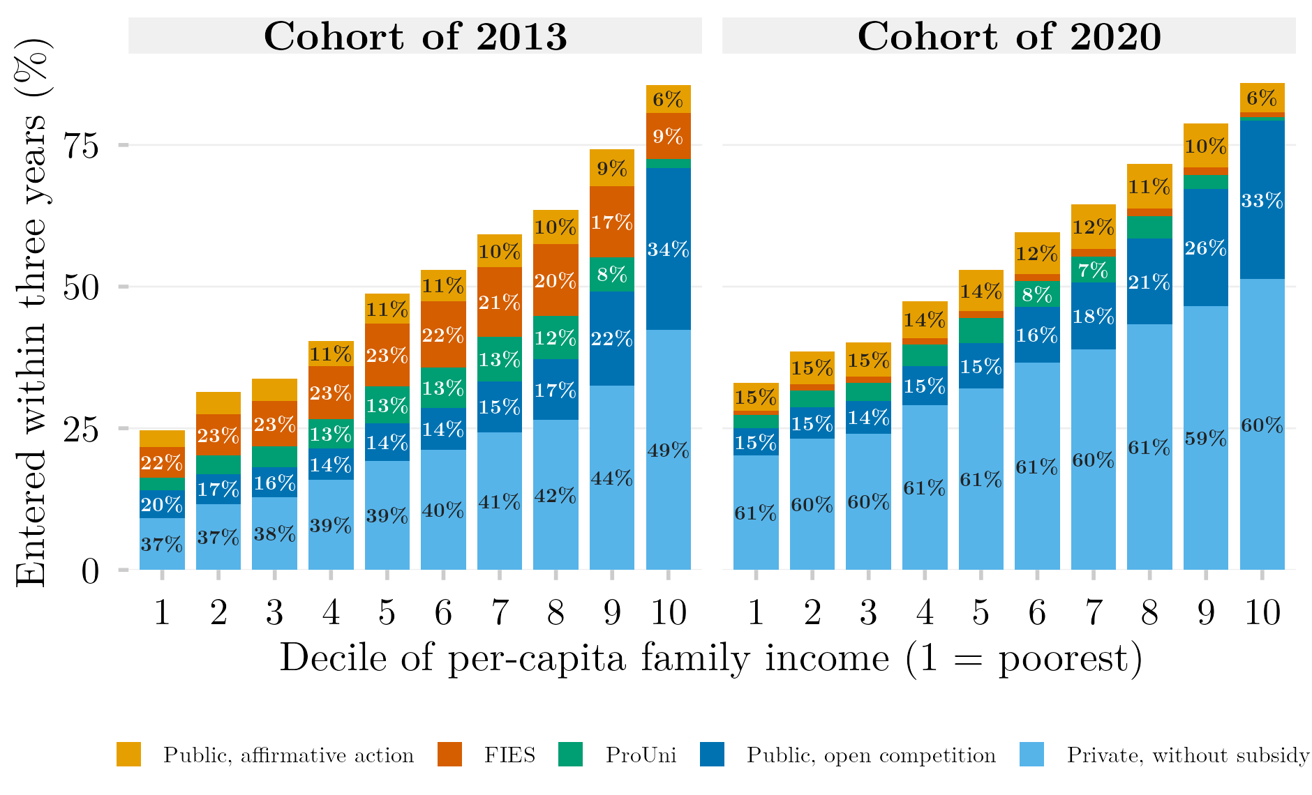
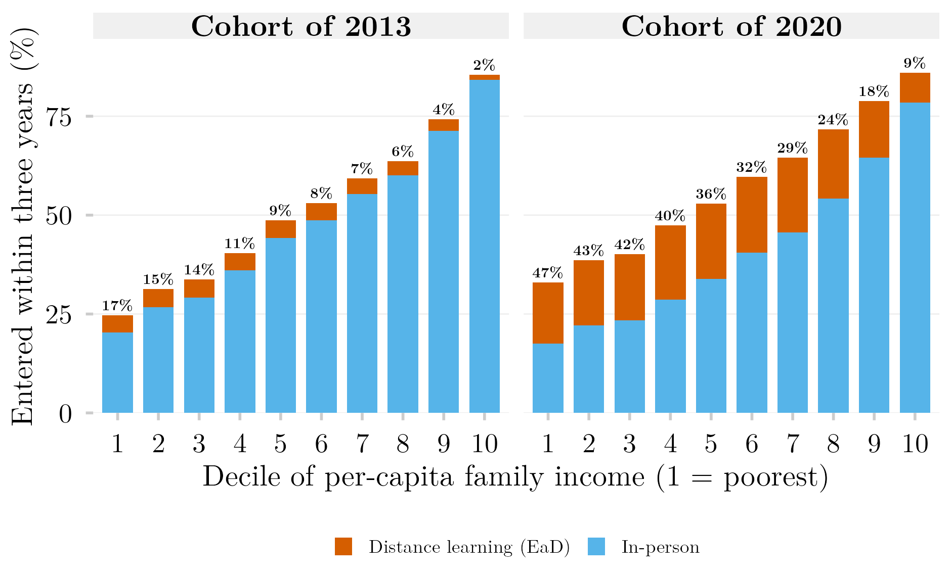
Size and location of the difference. Dropping the flag adds about 55,000 entrants to the 2013 cohort (8.7% more) and 41,000 to the 2020 cohort (8.2% more), against unchanged cohort totals. Total entry rises by 2.5 to 5.8 percentage points depending on the decile, with the largest gains in the middle of the distribution and the smallest in the richest decile. Almost all of the added entrants fall in two segments. In the route figure, unsubsidised private entry rises by 2.8 to 4.4 points in the lower seven deciles of both cohorts, while ProUni and FIES move by less than half a point. In the mode figure, distance-learning entry in the 2020 cohort rises by 4 to 5 points in the lower eight deciles; in the poorest decile it goes from 15.5% to 19.5%, and its share of that decile’s entrants from 46.9% to 51.7%.
Interpretation. The gap between the two definitions counts students who left their course within the entry year, before the census date. The segments where it concentrates — unsubsidised private study and, in 2020, distance learning — are those with no scholarship or loan tying the student to the course. Students on ProUni or FIES barely appear in the gap. The pattern agrees with the growth of records flagged IN_MATRICULA = 0 in the register as a whole, from 22.8% in 2011 to 32.6% in 2023 (RELATORIO.md). Transfers between institutions also enter the gap, so it cannot be read as a dropout rate. The substantive readings in the chapter survive the correction, and several become stronger: in-person entry still falls in every decile between the cohorts, the net gain in entry remains largest at the bottom and close to zero at the top, and the reserved-seat route still exceeds ProUni in every decile of the 2020 cohort.
Code. Both definitions are produced by the same scripts. 031_Extrair_ProUni_FIES.R and 054_Extrair_EaD.R extract without the flag by default and, with FILTRO_IN_MATRICULA=TRUE set in the environment, reproduce the old definition in files suffixed _com_in_matricula; 052_Fig_Portas_Renda_Empilhado.R and 055_Fig_Portas_Renda_EaD.R draw both versions.
B.8.16 Replication of Senkevics et al. (2024): Design, Estimation and Departures for the 2012 Cohort of @fig-replicacao-senkevics2024-coortes
Design. The cohort is every student enrolled in the final year of secondary education in the 2012 Censo Escolar (TP_ETAPA_ENSINO in 27, 28, 29, 32, 33, 34, 37, 38), aged 16–22, followed in the ENEM editions of 2012–2016 and in the Censo da Educação Superior of 2013–2017; a student counts as having entered if any first enrollment appears within those five years, and the sector is that of the earliest one (TP_CATEGORIA_ADMINISTRATIVA 1–3 public, 4–9 private). Performance is the mean of the four objective ENEM tests, without the essay, converted to deciles within the cohort. Family income per capita divides the midpoint of the declared income band (in minimum wages of the ENEM edition, deflated by the INPC to March 2023) by the declared number of household members, and is likewise cut into deciles within the cohort. Every one of these constants is taken from the authors’ replication package, with the source line recorded next to each in 4-DA-Code/2026-08_Replicacao_Senkevics2024/015_Especificacao.R; the package diverges from the article’s text on the deflator target (July 2023 on p. 864, March 2023 in the code), and the code was followed. The analytic sample is 977,450 students, against 1,133,027 in the article.
Estimation. The figure plots predicted probabilities from a multinomial logit of destination (no access, public, private) on the full interaction of income decile and performance decile, fitted with nnet::multinom on the 300-cell contingency table with cell counts as weights. This is the authors’ own reduced specification (reg_standard in their code). With ten income deciles fully interacted with ten performance deciles and three outcomes, the model has one parameter per cell and is saturated, so the predicted probabilities coincide with the observed cell proportions; the published figure instead reports probabilities from a model that adds sex, colour, a quadratic in age, school network, rural location, state and ENEM edition, which is why its levels differ where composition differs most between income strata. Circle area is the conditional distribution of performance within each income decile, following the article’s convention that circles of one colour sum to one within a panel.
Departures from the original, all forced by the data access layer. The SEDAP+ platform returns only aggregate queries under differential privacy (\(\varepsilon = 1\)), which rules out the following operations of the authors’ code. (D1) The cohort is students enrolled in the final year, since the completion flag (IN_CONCLUINTE) is not in the linked project; the authors use approved completers. (D2) The eight controls of the published model are omitted, because the contingency table they require has on the order of \(10^8\) cells against a query limit of roughly five grouping columns with suppression of small cells. (D3) A student who sat the ENEM more than once is assigned the last edition taken; the authors’ primary rule, the edition immediately preceding enrollment, needs per-individual aggregation, which the privacy layer forbids, so only their fallback rule (ultimoenem) is available. (D4) The authors’ random tie-breaker for students with several simultaneous enrollment records is not applied; the earliest enrollment year decides. (D5) Cell counts carry differential-privacy noise; the row-loss reported by the platform was zero in every query, and re-running the same query gives cell counts that differ by about three students on average (at most 27). (D6) The income band is anchored to the minimum-wage value printed in each edition’s questionnaire rather than to the legal minimum wage of that year; the two coincide for 2012–2016, so this affects none of the numbers here and matters only for the later cohorts of the same pipeline. (D7) Students with no socio-economic questionnaire, and therefore no income, are excluded, as they are by construction in the authors’ Stata code; they are 330 students (0.03%) in this cohort, all from the 2015 and 2016 editions, in which the questionnaire first admitted blank answers. Until 2026-09-14 the pipeline’s decile expression assigned these students to the top income decile; the error was found by querying the composition of that decile and is documented in sec-fignote-replicacao-senkevics2024-coortes, where it matters.
Validation. Marginals against the article: 74.8% private and 25.2% public among entrants (published: 75.8% and 24.2%); 67.1% of the cohort entering within five years (published: 68.9%). Cell-level readings of the printed figure were compared with the replication at the four corners of the grid; the largest gap is the public-sector probability for the poorest income decile at the top performance decile (0.65 here, roughly 0.40 published), consistent with the omitted controls absorbing the composition of that small cell.
Related figures not promoted. The same pipeline extends the design to the secondary-school cohorts of 2014, 2017 and 2019 and applies the article’s two decompositions (equations 3 and 4) to all four cohorts; those figures and the diagnostics on ENEM participation by school network and on the comparability of the ENEM income variable across editions remain in 6-images-tables/graphs/replicacao-senkevics2024/ and are documented in NEWS.md (entries of 2026-08-07 and 2026-08-08). The 2012 cohort is the only one that is a replication in the strict sense — the only one for which published numbers exist to validate against — and is the one this entry describes; Figure fig-replicacao-senkevics2024-coortes shows it alongside the 2019 cohort, whose own entry follows (sec-fignote-replicacao-senkevics2024-coortes). Reproduce: posts/replicacao-senkevics2024-coortes/ (Open Data Analysis).
B.8.17 The 2012 and 2019 Cohorts Compared (@fig-replicacao-senkevics2024-coortes)
Design. Identical to the 2012 replication (sec-replicacao-senkevics2024-design) for each cohort separately: the 2019 cohort is every student in the final year of secondary education in the 2019 Censo Escolar, aged 16–22, followed in the ENEM editions of 2019–2023 and in the Censo da Educação Superior of 2020–2024. Income and performance deciles are cut within each cohort, so a decile is a relative position among that cohort’s examinees, not a fixed level of income or score; the deflated income cut-points move little between the two cohorts (the boundary of the first decile sits at R$249 in 2012 and R$256 in 2019, in March-2023 prices), but this stability reflects the questionnaire’s income bands, which are anchored to the minimum wage, more than the income distribution itself. Departures D1–D7 apply unchanged, with D6 relevant only to the 2022 and 2023 editions and D7 excluding 2,091 students (0.28%) without a questionnaire. The 2019 analytic sample is 746,852 students in 300 cells.
Coverage and the selection it implies. The analytic sample is the subset of the school cohort that sat all four objective ENEM tests in at least one edition of the five-year window and could be linked by masked CPF. It covers 44.9% of the 2012 cohort (977,450 of 2,175,504 final-year enrollments) and 35.0% of the 2019 cohort (746,852 of 2,132,311). The decline has two sources visible in the data: the share of the cohort with a linkable CPF falls from 87% to 76%, and ENEM participation collapsed in the pandemic editions — the raw linkage of the 2019 cohort to the ENEM of 2021 and 2022 is 13% and 8% of the students with a CPF, against 30% and 24% for the corresponding editions (2014 and 2015) of the 2012 cohort. Because the deciles are cut within the observed sample, a change in who sits the examination changes what “first decile” means between cohorts. The direction of the resulting bias is not identifiable from these data alone; the diagnostic on participation by school network (130_Diagnostico_Selecao_ENEM.R) shows that participation diverged between the state and private school networks over the same window, which is the channel most likely to matter, since the network a student comes from is itself a strong proxy for income.
Holding the school network fixed. The check that this channel permits is to repeat the comparison within a single network of origin, where every student was exposed to the same kind of school and the same drift in examination participation. The matrix was therefore re-extracted with the school’s administrative dependency (TP_DEPENDENCIA) as a fourth dimension (150_Extrair_Por_Rede.R, 160_Analise_Por_Rede.R; departures D1–D7 as above, with the global decile cut-points of each cohort kept so that the same income positions are compared). Within the state network, which holds 95,172 of the poorest decile’s 2012 students and 54,195 of its 2019 students, the gap in non-access between the poorest and the richest income deciles falls from 32.3 to 23.5 percentage points on average across performance deciles, and falls in every one of the ten (from 48.6 to 40.9 at the lowest performance decile, 37.0 to 22.8 at the sixth, 9.7 to 5.1 at the ninth). Within the private network the average gap falls from 21.1 to 14.7. A change in which networks’ students sit the examination cannot produce a fall inside a network, so the decline between the cohorts is not only a change of composition between them; the size of the within-network fall (8.8 points in the state network, against 10.7 for the income gradient in the pooled sample) is the better estimate of how much of it is real. These by-network cells are sparser than the pooled ones and the platform suppressed 4–12% of rows in each query, so the figures are reported here rather than drawn.
The edition rule. Under departure D3, a student who sat the ENEM more than once is scored on the last edition taken. The mix of editions differs sharply between cohorts: 37% of the 2012 sample is scored on the edition of the school-leaving year and 23% on the edition four years later, against 59% and 8.5% for 2019, a consequence of the collapse of ENEM participation in the pandemic editions. Restricting both cohorts to students scored on the school-leaving edition leaves the result intact: the income gap in non-access, weighted by cell size, falls by 16.3 percentage points between the cohorts against 16.0 on the full sample, and the gap at each performance decile moves by similar amounts under either rule.
How departure D7 was found. A first version of this figure (2026-09-14, superseded the same day) showed the cell of the richest income decile at the lowest performance decile as the only one of the hundred cells in which non-access did not decrease with income, with non-access rising from 30% in 2012 to 47% in 2017 and 41% in 2019. Querying the composition of that cell by declared income band and household size (170_Verificar_Figura_SEDAP.R) showed that in the 2023 edition 83% of it consisted of students with no socio-economic questionnaire, whom the pipeline’s decile expression — a CASE whose final ELSE branch returned the top decile — had assigned to the richest decile. These students, who sat the examination late and without filling in the questionnaire, have very low scores and very low enrollment, and there were 360 of them in the 2012 cohort against 2,091 in 2019, which is why the artefact grew across cohorts. After their exclusion the cell falls back onto the monotone curve (non-access 25%, 25%, 21% and 19% across the four cohorts), and the earlier reading of a collapse in the income gap at the lowest performance decile disappears with it: the gap there falls from 58 to 49 points, in line with the neighbouring deciles.
What changes and what does not. Sampling precision is not a constraint: the smallest cell in the figure has 749 students, every 95% Wilson interval is narrower than ±3.3 percentage points, and the noise added by the differential-privacy layer (ε = 1), measured by re-running the same query and comparing cell counts, has a standard deviation of about three students per cell (the largest observed deviation was 27), which is 0.4 points in the smallest cell of the figure and below 0.1 in a typical one. Of the sixty stratum-by-performance-by-destination cells, 50 differ significantly between 2012 and 2019 at the 5% level; the exceptions are cells of the richest decile that were already near zero or near their ceiling, and the smallest cell of the poorest decile. The change is concentrated in the poorest decile and in the private sector: its probability of non-access falls by 14–18 points across performance deciles 1–7, its probability of private-sector entry at the lowest performance decile doubles (14% to 28%), and its probability of public-sector entry rises in every performance decile, by 2–5 points at the extremes and by 9–13 points in deciles 6–9. The richest decile moves little in any panel. Two consequences follow for how the figure can be read. First, both the gradient of access over performance and the gradient over income flatten between the cohorts, and the income gradient flattens somewhat more (from 37 to 27 points, averaged over performance deciles, a fall of 29%, against 52 to 40 points for the performance gradient averaged over income deciles, a fall of 23%), so relative to income, access became if anything more tied to performance, not less; what fell is the weight of income. Second, the performance gradient within the public sector is unchanged at 61–63 points in every cohort, while within the private sector it turned from mildly negative to clearly negative (−9 to −22 points): the sector that absorbed the poorest decile’s gain is the one whose intake is least tied to the examination. The figure cannot separate in-person from distance enrollment within the private sector, which is the most likely mechanism and requires a separate extraction. Replication code: 4-DA-Code/2026-08_Replicacao_Senkevics2024/085_Fig_Coortes_2012_2019_Apendice.R; diagnostics summarized in NEWS.md, entry of 2026-09-14. Reproduce: posts/replicacao-senkevics2024-coortes/ (Open Data Analysis).