Introduction to educabr2 • educabr2

library(educabr2)

About the package

educabr2 provides, under a single canonical tidy schema, the most extensive set of harmonised historical series on Brazilian education available in analytic format:

Tertiary (higher-education) enrollment — 1907 to 2024, 118 years of coverage, drawing on seven distinct primary sources (IBGE Statistics of the 20th Century, Durham, Maduro Junior, Kang, INEP Synopsis, INEP Microdata, and the INEP CENSUP Power BI panel).
Compulsory (fundamental) and upper-secondary enrollment — 1933 to 2010, with race/colour disaggregation from 1960 onwards (Kang, Paese & Felix 2021).
Mean years of schooling of the adult population — 1925 to 2015, with breakdowns by sex, race/colour, macroregion and state (Walter & Kang 2024).
Public expenditure on education — 1933 to 2010, share of GDP by stage, per-student spending as share of GDP per capita, and the Kang & Menetrier (2024) “double ratio” indicators of fiscal regressivity.
Grade-progression ratio (GDR6) — 1955 to 2010, BR + 20 UFs, a proxy for early-primary retention drawn from Kang, Paese & Felix (2021).
International educational attainment — 1870 to 2010, 111 countries, shares of the population aged 15-64 that completed primary, secondary and tertiary education, with sex breakdowns (Lee & Lee 2016) — so the Brazilian trajectory can be read against the world record without leaving the package.

Every transformation is auditable: each output row carries a canonical source key (catalogued in inst/dict/vocabularies/sources.yaml) and a source_note with the exact table or chapter of origin.

Installation

# From GitHub
remotes::install_github("mancano-tales/educabr2")

A five-function API

The public interface is intentionally minimal — one function per theme, all returning tibbles in the same canonical long schema:

# Schemas of the five return shapes
str(get_enrollment(level = "fundamental", year = 1950))
#> tibble [2 × 16] (S3: tbl_df/tbl/data.frame)
#>  $ year            : int [1:2] 1950 1950
#>  $ geo_level       : chr [1:2] "BR" "BR"
#>  $ geo_code        : chr [1:2] "BR" "BR"
#>  $ geo_name        : chr [1:2] "Brasil" "Brasil"
#>  $ level           : chr [1:2] "fundamental" "fundamental"
#>  $ network         : chr [1:2] "total" "total"
#>  $ institution_type: chr [1:2] "total" "total"
#>  $ modality        : chr [1:2] "total" "total"
#>  $ dim_race        : chr [1:2] "total" "total"
#>  $ age_group       : chr [1:2] "7-14" NA
#>  $ indicator       : chr [1:2] "enrollment_rate" "enrollment_count"
#>  $ value           : num [1:2] 4.55e+01 4.73e+06
#>  $ unit            : chr [1:2] "percent" "count"
#>  $ source          : chr [1:2] "kang_paese_felix_2021" "kang_paese_felix_2021"
#>  $ source_note     : chr [1:2] "Kang, Paese & Felix (2021). RHE 39(2):191-218. doi:10.1017/S0212610921000112" "Kang, Paese & Felix (2021). RHE 39(2):191-218. doi:10.1017/S0212610921000112"
#>  $ is_derived      : logi [1:2] FALSE FALSE
#>  - attr(*, "educabr_meta")=List of 4
#>   ..$ build_script   : chr "data-raw/01_build_enrollment_kang_fgv.R"
#>   ..$ built_at       : POSIXct[1:1], format: "2026-05-18 09:38:50"
#>   ..$ primary_sources: chr [1:4] "kang_menetrier_comim_2024" "kang_paese_felix_2021" "kang_paese_felix_2021" "kang_menetrier_2024"
#>   ..$ raw_files      : chr [1:4] "data-raw/sources/kang_fgv_ibre_2023/1._matricula_primario_1871_2010_v_abril2023.xlsx" "data-raw/sources/kang_fgv_ibre_2023/2._matriculas_txmatriculas_porcor_1960_2010_v_abril2023.xlsx" "data-raw/sources/kang_fgv_ibre_2023/4._matricula_txmatriculas_1933_2010_v_abril2023.xlsx" "data-raw/sources/kang_fgv_ibre_2023/6._matricula_txmatriculas_estado_1955_2010_v_abril2023.xlsx"
str(get_schooling(year = 1950))
#> tibble [1 × 12] (S3: tbl_df/tbl/data.frame)
#>  $ year       : int 1950
#>  $ geo_level  : chr "BR"
#>  $ geo_code   : chr "BR"
#>  $ geo_name   : chr "Brasil"
#>  $ dim_race   : chr "total"
#>  $ dim_sex    : chr "total"
#>  $ age_group  : chr NA
#>  $ indicator  : chr "mean_years_schooling"
#>  $ value      : num 1.59
#>  $ unit       : chr "years"
#>  $ source     : chr "walter_kang_2023"
#>  $ source_note: chr "Walter, J., & Kang, T. H. (2024). A new dataset of average years of schooling in Brazil, 1925-2015. Economic Hi"| __truncated__
#>  - attr(*, "educabr_meta")=List of 5
#>   ..$ build_script  : chr "data-raw/02_build_schooling_kang_fgv.R"
#>   ..$ built_at      : POSIXct[1:1], format: "2026-07-10 01:00:11"
#>   ..$ primary_source: chr "walter_kang_2023"
#>   ..$ citation      : chr "Walter, J., & Kang, T. H. (2024). A new dataset of average years of schooling in Brazil, 1925-2015. Economic Hi"| __truncated__
#>   ..$ raw_files     : chr "data-raw/sources/kang_fgv_ibre_2023/3._anos_estudo_1925_2015_v_abril2023.xlsx"
str(get_expenditure(level = "total", indicator = "share_gdp", year = 1950))
#> tibble [1 × 13] (S3: tbl_df/tbl/data.frame)
#>  $ year       : int 1950
#>  $ geo_level  : chr "BR"
#>  $ geo_code   : chr "BR"
#>  $ geo_name   : chr "Brasil"
#>  $ level      : chr "total"
#>  $ network    : chr "publica"
#>  $ dim_race   : chr "total"
#>  $ age_group  : chr NA
#>  $ indicator  : chr "expenditure_share_gdp"
#>  $ value      : num 1.53
#>  $ unit       : chr "percent_gdp"
#>  $ source     : chr "kang_menetrier_2024"
#>  $ source_note: chr "Kang & Menetrier (2024). Estudos Econômicos 54(3). doi:10.1590/1980-53575434tkim"
#>  - attr(*, "educabr_meta")=List of 5
#>   ..$ build_script  : chr "data-raw/04_build_expenditure_kang_fgv.R"
#>   ..$ built_at      : POSIXct[1:1], format: "2026-05-19 02:42:48"
#>   ..$ primary_source: chr "kang_menetrier_2024"
#>   ..$ citation      : chr "Kang & Menetrier (2024). Estudos Econômicos 54(3). doi:10.1590/1980-53575434tkim"
#>   ..$ raw_files     : chr "data-raw/sources/kang_fgv_ibre_2023/5._despesa_pub_educ_1933_2010_v_abril2023.xlsx"
str(get_progression(year = 1980))
#> tibble [1 × 13] (S3: tbl_df/tbl/data.frame)
#>  $ year       : int 1980
#>  $ geo_level  : chr "BR"
#>  $ geo_code   : chr "BR"
#>  $ geo_name   : chr "Brasil"
#>  $ level      : chr "fundamental_anos_iniciais"
#>  $ network    : chr "total"
#>  $ dim_race   : chr "total"
#>  $ age_group  : chr NA
#>  $ indicator  : chr "gross_distribution_ratio_grade_6"
#>  $ value      : num 0.461
#>  $ unit       : chr "ratio"
#>  $ source     : chr "kang_paese_felix_2021"
#>  $ source_note: chr "Kang, Paese & Felix (2021). RHE 39(2):191-218. doi:10.1017/S0212610921000112"
#>  - attr(*, "educabr_meta")=List of 5
#>   ..$ build_script  : chr "data-raw/05_build_progression_kang_fgv.R"
#>   ..$ built_at      : POSIXct[1:1], format: "2026-05-19 02:43:16"
#>   ..$ primary_source: chr "kang_paese_felix_2021"
#>   ..$ citation      : chr "Kang, Paese & Felix (2021). RHE 39(2):191-218. doi:10.1017/S0212610921000112"
#>   ..$ raw_files     : chr "data-raw/sources/kang_fgv_ibre_2023/7._gdr6_1955_2010_v_abril2023.xlsx"
str(get_attainment(geo = "BRA", year = 1950))
#> tibble [3 × 12] (S3: tbl_df/tbl/data.frame)
#>  $ year       : int [1:3] 1950 1950 1950
#>  $ geo_level  : chr [1:3] "country" "country" "country"
#>  $ geo_code   : chr [1:3] "BRA" "BRA" "BRA"
#>  $ geo_name   : chr [1:3] "Brazil" "Brazil" "Brazil"
#>   ..- attr(*, "label")= chr "Country name"
#>   ..- attr(*, "format.stata")= chr "%20s"
#>  $ level      : chr [1:3] "primary" "secondary" "tertiary"
#>  $ dim_sex    : chr [1:3] "total" "total" "total"
#>  $ age_group  : chr [1:3] "15-64" "15-64" "15-64"
#>  $ indicator  : chr [1:3] "attainment_share_completed" "attainment_share_completed" "attainment_share_completed"
#>  $ value      : num [1:3] 23.611 4.345 0.519
#>  $ unit       : chr [1:3] "percent" "percent" "percent"
#>  $ source     : chr [1:3] "lee_lee_2016" "lee_lee_2016" "lee_lee_2016"
#>  $ source_note: chr [1:3] "Lee, J.-W., & Lee, H. (2016). Human capital in the long run. Journal of Development Economics, 122, 147-169. do"| __truncated__ "Lee, J.-W., & Lee, H. (2016). Human capital in the long run. Journal of Development Economics, 122, 147-169. do"| __truncated__ "Lee, J.-W., & Lee, H. (2016). Human capital in the long run. Journal of Development Economics, 122, 147-169. do"| __truncated__
#>  - attr(*, "educabr_meta")=List of 5
#>   ..$ build_script  : chr "data-raw/06_build_lee_lee_2016.R"
#>   ..$ built_at      : POSIXct[1:1], format: "2026-05-25 16:54:26"
#>   ..$ primary_source: chr "lee_lee_2016"
#>   ..$ citation      : chr "Lee, J.-W., & Lee, H. (2016). Human capital in the long run. Journal of Development Economics, 122, 147-169. do"| __truncated__
#>   ..$ raw_files     : chr "https://barrolee.github.io/BarroLeeDataSet/LeeLee/LeeLee_v1.dta"

All five return long-format tibbles that follow the same canonical schema (inst/dict/schema.yaml), with columns for the geographic unit, the inequality dimension (race, sex, …), the source, and the value. The shared filters (year, geo_level, geo, source, wide, lang) work identically across the family. Because every function returns the same column set (constant-valued columns are kept where a source has no breakdown), results from different themes can be stacked directly with rbind()/bind_rows().

Note that the dimension argument is deliberately asymmetric: get_schooling() offers race and sex; get_enrollment() race only; get_attainment() sex only; get_expenditure() and get_progression() none. These asymmetries reproduce the physical limits of the historical sources, not limitations of the package.

Case 1 — gross enrollment rate by race/colour

Using dimension = "race" we can trace the trajectory of gross fundamental-education enrollment for the five IBGE race/colour categories between 1960 and 2010:

fund_race <- get_enrollment(
  level     = "fundamental",
  indicator = "rate",
  geo_level = "BR",
  dimension = "race",
  year      = c(1960, 2010)
)

head(fund_race)
#> # A tibble: 6 × 16
#>    year geo_level geo_code geo_name level      network institution_type modality
#>   <int> <chr>     <chr>    <chr>    <chr>      <chr>   <chr>            <chr>   
#> 1  1960 BR        BR       Brasil   fundament… total   total            total   
#> 2  1961 BR        BR       Brasil   fundament… total   total            total   
#> 3  1962 BR        BR       Brasil   fundament… total   total            total   
#> 4  1963 BR        BR       Brasil   fundament… total   total            total   
#> 5  1964 BR        BR       Brasil   fundament… total   total            total   
#> 6  1965 BR        BR       Brasil   fundament… total   total            total   
#> # ℹ 8 more variables: dim_race <chr>, age_group <chr>, indicator <chr>,
#> #   value <dbl>, unit <chr>, source <chr>, source_note <chr>, is_derived <lgl>

The gap between the three main categories (white, black, brown) traces one of the central narratives in the sociological literature on Brazilian education — relative convergence at compulsory levels alongside persistent inequality at higher levels.

Case 2 — multi-source comparison for tertiary enrollment

Brazilian tertiary enrollment has been reconstructed by multiple authors with slightly different methodologies, especially for the long 1933–2000 period when official sources are sparse. The educabr2 package keeps all competing estimates side by side, enabling direct comparison:

ter_1980 <- get_enrollment(
  level     = "superior",
  year      = 1980,
  network   = "total",
  modality  = "total",
  indicator = "count"
)

ter_1980[, c("source", "value", "source_note")]
#> # A tibble: 4 × 3
#>   source                  value source_note                                     
#>   <chr>                   <dbl> <chr>                                           
#> 1 kang_paese_felix_2021 1377286 Kang, Paese & Felix (2021). RHE 39(2):191-218. …
#> 2 durham_2005           1377286 Durham (2005). Educação superior, pública e pri…
#> 3 kang_paese_felix_2021 1377286 Kang, Paese & Felix (2021), RHE 39(2):191-218. …
#> 4 maduro_junior_2007    1377286 Maduro Junior (2007). Taxas de matrícula e gast…

For 1980 several sources converge on the same value (~1.38 million), which suggests a stabilised figure in the literature. For other years estimates diverge — passing source = "..." to get_enrollment() is the recommended way to pin down a single series for secondary analysis.

When a single continuous series is needed instead of the full side-by-side panel, the package’s documented deduplication hierarchy gives the recommended order of precedence for overlapping years: INEP CENSUP microdata (2009-2024), then the INEP statistical synopses (1995-2008), then Kang, Paese & Felix (1990-1994), then Maduro Junior, then Durham, and finally the IBGE Statistics of the 20th Century. The most disaggregated and official source available always wins.

Case 3 — the reconstructed totals problem (2000-2008)

Between 2000 and 2008 INEP began collecting distance-learning (EAD) enrollment in a separate CENSUP table (tabela7.x), but did not add it to the total of in-person enrollment published in tabela5.x. This means that headline “total” series for that interval published by Kang, Durham, Maduro Junior, and INEP’s own synopsis are systematically undercounted — by up to ~700,000 enrollments in 2008 by our reckoning.

From 2009 onwards the CENSUP microdata already aggregate in-person and EAD in the same registry, and the problem resolves itself.

For this transition interval, educabr2 ships reconstructed totals that combine the in-person component of each source with INEP’s published EAD figures. These rows carry is_derived = TRUE and are excluded from the default get_enrollment() output; pass include_derived = TRUE to inspect them:

recon <- get_enrollment(
  level           = "superior",
  year            = c(2000, 2008),
  network         = "total",
  modality        = "total",
  indicator       = "count",
  include_derived = TRUE
)

recon[recon$is_derived, c("year", "source", "value")]
#> # A tibble: 23 × 3
#>     year source                                      value
#>    <int> <chr>                                       <dbl>
#>  1  2000 durham_2005+inep_sinopse_censup           2695927
#>  2  2000 inep_sinopse_censup+inep_sinopse_censup   2695927
#>  3  2000 kang_paese_felix_2021+inep_sinopse_censup 2695927
#>  4  2000 maduro_junior_2007+inep_sinopse_censup    2695927
#>  5  2001 durham_2005+inep_sinopse_censup           3045113
#>  6  2001 inep_sinopse_censup+inep_sinopse_censup   3036113
#>  7  2001 inep_sinopse_censup+inep_sinopse_censup   3036113
#>  8  2001 kang_paese_felix_2021+inep_sinopse_censup 3036113
#>  9  2001 maduro_junior_2007+inep_sinopse_censup    3036113
#> 10  2003 inep_sinopse_censup+inep_sinopse_censup   3936933
#> # ℹ 13 more rows

The composite source key (e.g. kang_paese_felix_2021+inep_sinopse_censup) makes it explicit that this is a combination: the in-person component comes from the first source and the EAD component comes from the second. The source_note records the exact composition for citation purposes.

Suggested citation convention: “Reconstructed total computed from {in-person source} (in-person) and INEP CENSUP Synopsis (EAD), following the methodology documented in educabr2 (Mançano 2026).”

Case 4 — mean years of schooling by sex

schooling_sex <- get_schooling(
  geo_level = "BR",
  dimension = "sex"
)

tail(schooling_sex)
#> # A tibble: 6 × 12
#>    year geo_level geo_code geo_name dim_race dim_sex age_group indicator   value
#>   <int> <chr>     <chr>    <chr>    <chr>    <chr>   <chr>     <chr>       <dbl>
#> 1  2010 BR        BR       Brasil   total    male    NA        mean_years…  8.03
#> 2  2011 BR        BR       Brasil   total    male    NA        mean_years…  8.2 
#> 3  2012 BR        BR       Brasil   total    male    NA        mean_years…  8.39
#> 4  2013 BR        BR       Brasil   total    male    NA        mean_years…  8.49
#> 5  2014 BR        BR       Brasil   total    male    NA        mean_years…  8.63
#> 6  2015 BR        BR       Brasil   total    male    NA        mean_years…  8.72
#> # ℹ 3 more variables: unit <chr>, source <chr>, source_note <chr>

This series captures the historical reversal of the gender gap: in 1925 men averaged more years of schooling than women; over the 20th century that advantage inverts, and by 2015 women surpass men in average attainment.

Case 5 — fiscal regressivity in education spending

Kang & Menetrier (2024) operationalise a long-standing claim of the political economy of Brazilian education — that the State spends disproportionately more per tertiary student than per primary student — through their double ratio indicator: per-student public spending on Ensino Superior divided by per-student public spending on EF1 (anos iniciais).

ratio <- get_expenditure(indicator = "double_ratio_es_ef1")
ratio[ratio$year %in% c(1933, 1960, 1980, 2000, 2010),
      c("year", "value")]
#> # A tibble: 5 × 2
#>    year value
#>   <int> <dbl>
#> 1  1933 66.0 
#> 2  1960 86.6 
#> 3  1980 15.9 
#> 4  2000 16.8 
#> 5  2010  8.36

In 1933 the State spent roughly 66 times more per tertiary student than per first-grade student. By 2010 that ratio had fallen to under 9. The series shows that the historical trajectory of fiscal expansion in basic education during the second half of the 20th century did meaningfully reduce regressivity — though it never eliminated it.

Case 6 — early-primary retention (GDR6)

The GDR6 (Gross Distribution Ratio for grade 6) — defined as the ratio of enrollment in grades 4–6 to enrollment in grades 1–3 of the old eight-year primary system — is a flow indicator of how many children make it past the early primary grades. Higher values mean fewer dropouts and repeaters in the lower grades.

gdr_states <- get_progression(
  geo_level = "UF",
  geo       = c("SP", "BA"),
  year      = c(1955, 2010)
)

gdr_states[gdr_states$year %in% c(1960, 1980, 2000, 2010),
           c("year", "geo_code", "value")]
#> # A tibble: 8 × 3
#>    year geo_code value
#>   <int> <chr>    <dbl>
#> 1  1960 BA       0.187
#> 2  1980 BA       0.276
#> 3  2000 BA       0.649
#> 4  2010 BA       0.848
#> 5  1960 SP       0.273
#> 6  1980 SP       0.665
#> 7  2000 SP       1.09 
#> 8  2010 SP       0.952

The persistent SP-vs-BA gap is one of the canonical illustrations of regional inequality in the historical literature: in 1960 the SP/BA ratio is already wide, and only narrows substantially after the 1990s reforms.

UF coverage caveat. Kang, Paese & Felix’s compilation covers 20 federation units (AL, AM, BA, CE, ES, GO, MA, MG, MT, PA, PB, PE, PI, PR, RJ, RN, RS, SC, SE, SP). Newer or territorial-origin states (AC, AP, DF, MS, RO, RR, TO) are not in the source. The BR national series has documented gaps at 1988-1990 and 1994 due to transitions in the official grade structure.

Case 7 — Brazil in international perspective

The Lee & Lee (2016) panel lets you place the Brazilian expansion against comparators without leaving the package:

att <- get_attainment(
  level = "tertiary",
  geo   = c("BRA", "ARG", "KOR", "USA"),
  year  = c(1950, 2010)
)

att[att$year %in% c(1950, 1980, 2010),
    c("year", "geo_code", "value")]
#> # A tibble: 12 × 3
#>     year geo_code  value
#>    <int> <chr>     <dbl>
#>  1  1950 ARG       0.737
#>  2  1980 ARG       3.71 
#>  3  2010 ARG       2.31 
#>  4  1950 BRA       0.519
#>  5  1980 BRA       2.90 
#>  6  2010 BRA       6.59 
#>  7  1950 KOR       0.748
#>  8  1980 KOR       4.89 
#>  9  2010 KOR      33.6  
#> 10  1950 USA       7.16 
#> 11  1980 USA      17.9  
#> 12  2010 USA      27.5

The built-in visualization system

The package ships a plotting toolkit designed after Kieran Healy’s Data Visualization principles, so that a query can become a publication-ready figure in three lines:

theme_educabr() — a serif, minimal theme; with plot_titles = FALSE it strips in-canvas titles for LaTeX/Quarto manuscripts where captions live in the document. If a local TinyTeX installation is found (and showtext/sysfonts are installed), the LaTeX font Latin Modern Roman is registered automatically.
scale_colour_educabr() / scale_fill_educabr() — the colorblind-safe Okabe-Ito palette.
scale_x_year_educabr(years) — a year axis for century-long series: break spacing follows the span of the data, and the first and last years present are always labelled.

library(ggplot2)

df <- get_schooling(geo_level = "BR", dimension = "sex")

ggplot(df, aes(year, value, colour = dim_sex)) +
  geom_line(linewidth = 0.9) +
  scale_colour_educabr(name = NULL) +
  scale_x_year_educabr(df$year) +
  theme_educabr() +
  labs(x = NULL, y = "Mean years of schooling",
       title = "The gender gap in schooling reversed over the 20th century")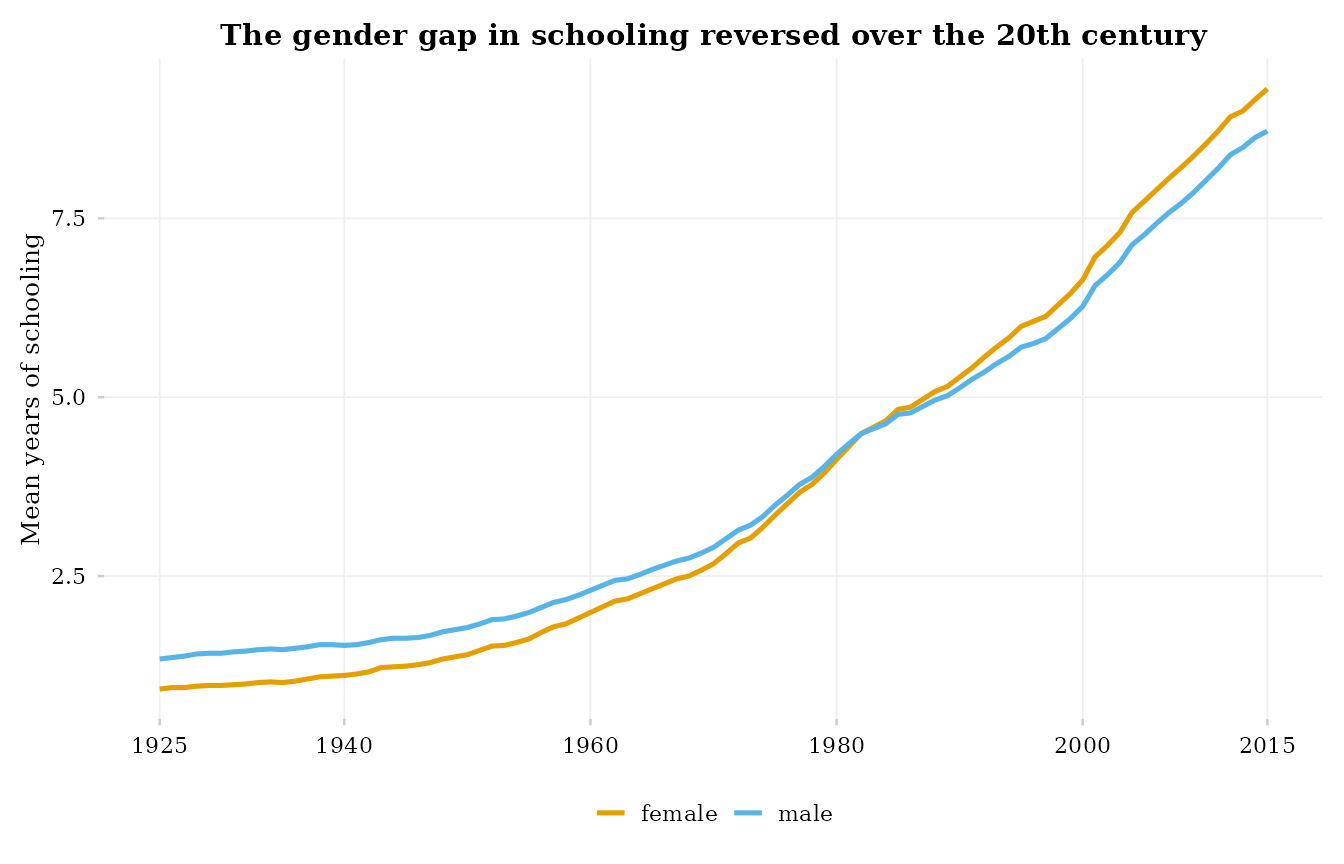

Interactive dashboard

The package ships a Shiny dashboard with a curated Overview tab (four story charts for non-technical audiences) plus six thematic tabs — one per theme (Enrollment, Tertiary Education, Educational Attainment, Public Expenditure, Grade Progression, International Comparison):

educabr2::run_dashboard()

The dashboard replicates the multi-source tertiary comparison and the expenditure / progression / international series interactively. Each tab has a “View R code” button that emits the educabr2 + ggplot2 snippet needed to reproduce the visualisation in your local R session — styled with the package’s own visualization system described above — a direct bridge between dashboard exploration and reproducible scripted analysis.

Sources and citation

Every series carries a canonical source key (source) with the full reference catalogued in inst/dict/vocabularies/sources.yaml. The seven primary tertiary sources are:

Kang, T. H., Paese, L. H. Z., & Felix, N. F. A. (2021). Late and unequal. Revista de Historia Económica 39(2), 191-218. doi:10.1017/S0212610921000112
Kang, T. H., & Menetrier, I. (2024). Políticas elitistas e despesas públicas em educação. Estudos Econômicos 54(3). doi:10.1590/1980-53575434tkim
Kang, T. H., Menetrier, I., & Comim, F. (2024). The side effects of a big push growth strategy. RHE 42(3), 387-414. doi:10.1017/S0212610924000120
Walter, J. R., & Kang, T. H. (2024). A new dataset of average years of schooling in Brazil. Economic History of Developing Regions 39(3), 307-336. doi:10.1080/20780389.2024.2417268
Durham, E. R. (2005). Educação superior, pública e privada. In Schwartzman (ed.), Os desafios da educação no Brasil, pp. 191-233.
Maduro Junior, P. R. R. M. (2007). Taxas de matrícula e gastos em educação no Brasil [MSc dissertation, FGV/EPGE]. hdl:10438/110
IBGE (2007). Estatísticas do Século XX. seculoxx.ibge.gov.br
INEP/MEC. Sinopse Estatística da Educação Superior (1995-2008).
INEP/MEC. Microdados do Censo da Educação Superior (2009-2024).
INEP/MEC. CENSUP Power BI panel (2010-2024).

The educabr_cite() helper turns any source key (or the source column of a query result) into a ready-to-paste reference:

educabr_cite("kang_paese_felix_2021", style = "text")
#> [1] "(2021). \"Kang, T. H., Paese, L. H. Z., & Felix, N. F. A. (2021). Late\nand unequal: Enrolments and retention in Brazilian education,\n1933-2010. Revista de Historia Económica / Journal of Iberian and Latin\nAmerican Economic History, 39(2), 191–218.\"\ndoi:10.1017/S0212610921000112\n<https://doi.org/10.1017/S0212610921000112>.\n<https://doi.org/10.1017/S0212610921000112>."

Use style = "bibtex" for a BibTeX entry, or call educabr_cite() with no arguments to list all bundled sources. Please cite both the package (for the harmonization) and the original compilations (for the archival work that produced the numbers).

To cite the package itself:

Mançano, T. (2026). educabr2: Harmonized Historical Series on Brazilian Education (version 0.1.0). https://github.com/mancano-tales/educabr2